The Mobile NAPL Interval, Part 2: Confined and Perched LNAPL
Volume 5, Issue 4 | December 2015

Download PDF

Applied NAPL Science Review

Demystifying NAPL Science for the Remediation Manager

Editor: J. Michael Hawthorne, PG
Asst. Editor: Dr. Rangaramanujam Muthu, PE

ANSR Scientific Advisory Board
J. Michael Hawthorne, PG, Board of Chairman, GEI Consultants Inc.
Mark Adamski, PG, BP Americas
Stephen S. Boynton, PE, LSP, Subsurface Env. Solutions, LLC
Dr. Randall Charbeneau, University of Texas
Paul Cho, PG, CA Regional Water Quality Control Board-LA
Robert Frank, RG, CH2M
Dr. Sanjay Garg, Shell Global Solutions (US) Inc.
Randy St. Germain, Dakota Technologies, Inc.
Dr. Dennis Helsel, Practical Stats
Dr. Terrence Johnson, USEPA
Andrew J. Kirkman, PE, BP Americas
Mark Lyverse, PG, Chevron Energy Technology Company
Mark W. Malander, ExxonMobil Environmental Services

Applied NAPL Science Review (ANSR) is a scientific ejournal that provides insight into the science behind the characterization and remediation of Non-Aqueous Phase Liquids (NAPLs) using plain English. We welcome feedback, suggestions for future topics, questions, and recommended links to NAPL resources. All submittals should be sent to the editor.

The Mobile NAPL Interval
Part 2: Confined and Perched LNAPL

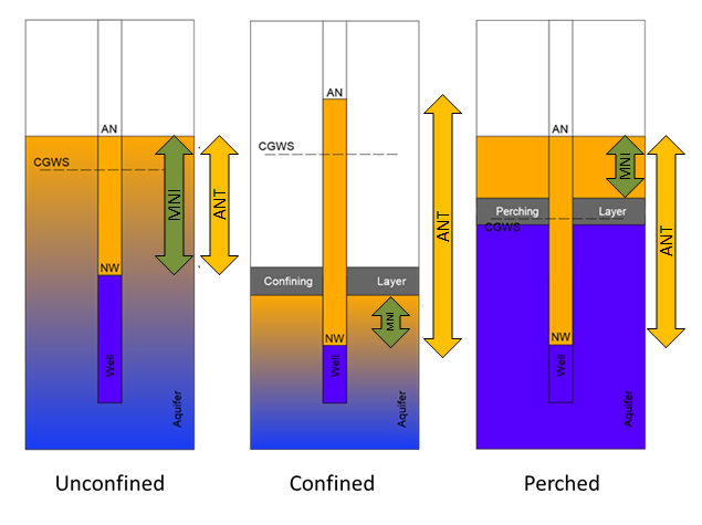
As discussed in Part 1 of this two part series, the mobile non-aqueous phase liquid (NAPL) interval (MNI) represents the thickness of the formation where NAPL is present above residual saturation. Generally this thickness can be thought of as the vertical extent corresponding to the “Shark Fin” portion of the total saturation profile. Understanding the location and extent of mobile light NAPL (LNAPL) is a critical element of the conceptual site model (CSM). This second article focuses on confined and perched LNAPL.

Under confined and perched LNAPL conditions, the MNI thickness and location are generally stable as the water table fluctuates because the MNI is trapped against the confining or perching layer and therefore vertically immobile. However, the apparent NAPL thickness (ANT) gauged in a well at equilibrium for confined and perched LNAPL is exaggerated and can be much larger than the MNI. Consequently, it is necessary to know the LNAPL hydrogeologic condition to understand the MNI.

Due to the stable MNI with groundwater fluctuations, the measured LNAPL transmissivity should be consistent over time as long as there is no change in LNAPL saturation due to migration or remediation.

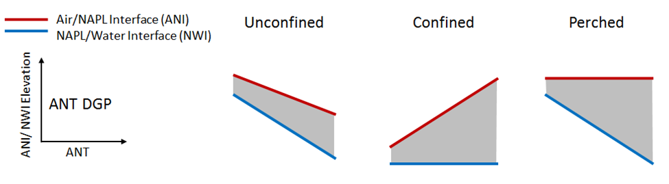
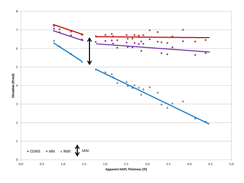
The hydrogeologic condition of the LNAPL can be identified using an ANT diagnostic gauge plot (DGP) of equilibrium gauging data (Kirkman et al, 2013; Hawthorne, 2011). Characteristic ANT DGP curves for unconfined, confined, and perched conditions are shown in Figure 2.

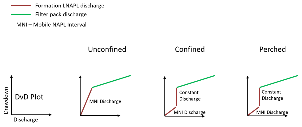
Discharge versus drawdown (DvD) plots generated from baildown tests or from gauged recharge data following manual skimming tests or oil/water ratio tests may also be used to identify the LNAPL hydrogeologic condition as well as the MNI (Kirkman et al, 2013; Hawthorne and Kirkman, 2011). Figure 3 shows characteristic DvD curves for unconfined, confined, and perched conditions.

Confined Conditions

Diagnostic Gauge Plots
The characteristic ANT DGP for confined conditions is a wedge shape where the NAPL/water interface (NWI) is constant and the air/NAPL interface (ANI) is increasing with increasing ANT (Figure 2). The NWI corresponds to the base of the MNI, but the confining contact (rather than the ANI) is the top of the MNI. The ANI will vary with changes in groundwater potentiometric surface (the calculated groundwater surface or CGWS), and may be substantially higher than the confining contact.

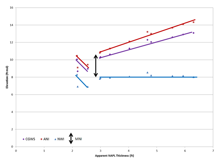
The confining contact can be identified on the ANT DGP if the equilibrium ANI has dropped below the elevation of the confining contact causing the NAPL condition to be temporarily unconfined. This change appears on the ANT DGP as an inflection point where the trend lines switch from the characteristic shape of confined conditions to that of unconfined conditions, and the ANI, CGWS, and NWI elevations all decrease with increasing ANT. The MNI for confined conditions corresponds to the equilibrium ANT at the inflection point on the DGP (Figure 4).

If the water table has not been low enough historically to identify the inflection point, the MNI can be estimated as the difference in elevation between the constant NWI and the confining contact identified from the boring log or other data in the CSM.

Discharge versus Drawdown Plots

The NAPL discharge rate on a DvD plot is constant when the NWI is above the confining contact. When the NWI drops below the confining contact, the NAPL in the well is in direct communication with the NAPL in the formation. For further increases in ANT, the NAPL drawdown and discharge rate linearly decrease as shown in Figure 5.

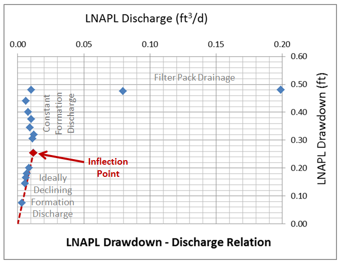
The confining contact can be identified as the elevation of the NWI when the NAPL discharge rate into the well begins to decrease linearly. The MNI is estimated as the elevation difference from the confining contact to the static NWI.

Perched Conditions

Diagnostic Gauge Plots

The characteristic ANT DGP for perched conditions is a wedge shape where the ANI is constant and the NWI elevation decreases with increasing ANT (Figure 2). The ANI corresponds to the top of the MNI, and the perching contact (not the NWI) is the bottom of the MNI. The NWI will vary with changes in the CGWS and may be well below the perching contact.

The perching contact can be identified on the ANT DGP if the equilibrium NWI has risen above the elevation of the perching contact causing the NAPL condition to be temporarily unconfined. The change can be identified on the DGP as an inflection point where the trend lines switch from the characteristic shape of perched conditions to that of unconfined conditions. The MNI for the perched conditions corresponds to the ANT at the inflection point on the DGP (Figure 6).

If the water table has not been high enough historically to identify the inflection point, the MNI can be estimated using the perching contact identified from the boring log or other data in the CSM. The MNI is the difference in elevation from the ANI to the perching contact.

Discharge versus Drawdown Plots

The NAPL discharge rate is constant when the ANI is below the perching contact. When the ANI rises above the perching contact, the NAPL in the well is in communication with the NAPL in the formation. For further increases in ANT, the NAPL drawdown and discharge rate linearly decrease as shown in Figure 5.

The perching contact can be identified as the elevation of the ANI when the NAPL discharge rate into the well begins to decrease linearly. The MNI is estimated as the elevation difference from the static ANI to the perching contact, and for perched NAPL is equal to the drawdown at the inflection point (Kirkman et al, 2013).

Summary
For confined and perched LNAPL the MNI cannot be estimated from the ANT gauged in a well at equilibrium, but can be derived from DGP and/or DvD plot analyses. For both confined and perched LNAPL, the MNI can be generally stable over time absent recovery, leaky boundaries, migration or the introduction of LNAPL from a “new” release. Because the MNI is stable, LNAPL transmissivity measurements should be stable over time as well. The MNI for confined and perched LNAPL (but not the ANT) represents the height of the “Shark Fin” saturation curve (i.e., the thickness of the formation with LNAPL present above residual saturation). Identification of the MNI is particularly critical for confined and perched LNAPL in order to correctly calculate LNAPL mobility and recoverability, to correctly model LNAPL saturation and recovery profiles, and to correctly target the portion of the formation with recoverable LNAPL.

A Word of Caution
DGPs require equilibrium fluid data. Use of non-equilibrium data can cause inaccurate estimation of MNI. A detailed CSM is required to understand which hydrogeologic condition is appropriate and how that condition has changed, or may change, over time. Estimated MNI should be verified against other lines of evidence in the CSM. Understanding MNI is critical for calculating NAPL drawdown and transmissivity. The final results need to be interpreted within the context of the precision of the MNI estimation.

References:
ASTM
2013 Standard Guide for Estimation of LNAPL Transmissivity. ASTM E2856-13. ASTM International, West Conshohocken, PA.

Hawthorne, J. Michael
2011 Diagnostic Gauge Plots, Applied NAPL Science Review (Volume 1, Issue 2), February 2011.

Hawthorne, J. Michael
2014 Calculating NAPL Drawdown, Applied NAPL Science Review, (Volume 4, issue 3), September 2014.

Hawthorne, J. Michael, and Andrew J. Kirkman
2011 Discharge vs. Drawdown Graphs, Applied NAPL Science Review (Volume 1, Issue 4), April 2011.

Kirkman, Andrew J., Mark Adamski, and J. Michael Hawthorne
2013 Identification and Assessment of Confined and Perched LNAPL Conditions, Groundwater Monitoring & Remediation, Volume 33, Issue 1, pp 75-86.

Research Corner

Thank you to Dr. Tom Sale of the Colorado State University, Center for Contaminant Hydrology, for
providing access to selected graduate level NAPL research.

A Mass Balance Approach to Resolving the Stability of LNAPL Bodies

Nicholas T. Mahler
Master of Science
Colorado State University

Abstract: Light non-aqueous phase liquids (LNAPLs) are commonly present in soils and groundwater beneath petroleum facilities. When sufficient amounts of LNAPL have been released continuous bodies of LNAPL form. These bodies can have detrimental impacts to soil gas and groundwater. Furthermore, with time they can expand or translate laterally. Measurements of LNAPL flux within continuous bodies typically indicate that LNAPL is moving, albeit slowly. Commonly, these fluxes have been used to infer (by continuity) that the bodies as a whole are expanding and/or translating laterally. In conflict with this, dissolved plumes downgradient of LNAPL bodies are widely thought to be stable or shrinking due to natural attenuation. The hypothesis of this research is that natural losses of LNAPL in contiguous bodies can play an important role in limiting expansion and/or lateral translation of LNAPL bodies. Much like dissolved phase plumes, LNAPL bodies can be stable when internal fluxes are balanced by natural losses.

As a first step, 50 measurements of LNAPL fluxes through wells from seven field sites are reviewed. All the values were acquired using tracer dilution techniques. The mean and median of the LNAPL flux measurements are 0.15 and 0.064 m/year, respectively. The measured LNAPL fluxes are three to five orders of magnitude less than typical groundwater fluxes. The primary significance of the small magnitude of the LNAPL fluxes relative to groundwater fluxes is that LNAPL discharge to the downgradient body could easily be equal to or less than the natural downgradient LNAPL losses that occur through dissolution into groundwater or evaporation into soil gas. In general no clear correlations are seen between measured LNAPL fluxes and LNAPL thicknesses in wells, lengths to downgradient edges of LNAPL, or the specific gravities (density of LNAPL/ density of water) of the LNAPL.

Secondly, a proof-of-concept sand tank experiment is presented. The objective was to resolve if natural LNAPL losses can limit expansion of an LNAPL body given a constant source. An open top glass and stainless steel tank (1 m by 0.5 m by 0.025 m) was filled with uniform coarse sand and water. Water was pumped through the tank producing a water seepage velocity of 0.25 m/day. Methyl tert-butyl ether (MTBE) was added to the tank at constant rates that were step-wise increased five times through a 120 day experiment. In all cases the MTBE body initially expanded followed by subsequent stabilization at a finite length. The key observation was that steady LNAPL pool lengths were achieved with a constant inflow of LNAPL into the system.

Lastly, analytical models are developed. The models describe the size of LNAPL bodies and spatial variations in LNAPL fluxes as a function of influent loading, rates of natural losses, and time. Three idealized geometries of LNAPL bodies are considered. These include one dimensional, circular, and oblong. Results indicate LNAPL fluxes decline progressing from the interior to the edges of an LNAPL body. Per the laboratory studies, the solutions show that LNAPL bodies with a constant source reach finite dimensions at large times. Building on this research it seems that a pragmatic goal for management of contiguous LNAPL bodies is attaining a condition where the LNAPL bodies as a whole are stable or shrinking.

The primary objective of ANSR is the dissemination of technical information on the science behind the characterization and remediation of Light and Dense Non-Aqueous Phase Liquids (NAPLs). Expanding on this goal, the Research Corner has been established to provide research information on advances in NAPL science from academia and similar research institutions. Each issue will provide a brief synopsis of a research topic and link to the thesis/dissertation/report, wherever available.

Practical Stats

Top Twelve Tip #7:
Maximize the Signal to Noise Ratio

Environmental data often come from ‘uncontrolled experiments’. Scientists must collect observational data rather than controlling all variables except one and examining only the effect of changes in the one. Effects of climate, weather, and human activities (among others) produce noise that can rarely be avoided or controlled. Whether performing hypothesis tests, regression, or trend analysis, it is important to account for the effects of uncontrolled variables that may be affecting the outcome of a statistical test.

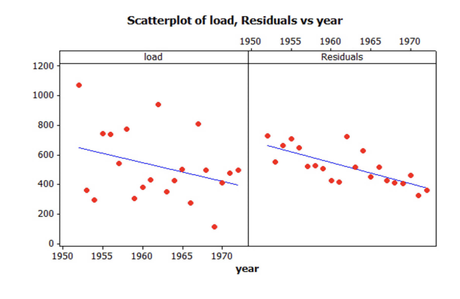
Load (mass) of sediment is plotted in the left panel below versus time. A simple regression produces a p-value of 0.15, insufficient for evidence of a linear relation between the two. Does this prove that there is no trend in load? No! Multiple regression removes the effect of streamflow, known by the scientist to be a major contributor to the pattern in load. The up and down variation in streamflow that causes some of the variation in load is removed, reducing the noise and making the trend signal easier to detect. This is pictured in the right-hand panel, where the trend signal can now be distinguished, resulting in a p-value <0.001. With environmental data, the scientist can rarely afford to do a simplistic test and stop there.