Mobile NAPL Interval Pt 1: Unconfined LNAPL
Volume 5, Issue 3 | Nov 2015

Download PDF

Applied NAPL Science Review

Demystifying NAPL Science for the Remediation Manager
Volume 5, Issue 3, November 2015

Editor: J. Michael Hawthorne, PG

Asst. Editor: Dr. Rangaramanujam Muthu, PE

ANSR Scientific Advisory Board
J. Michael Hawthorne, PG, Board of Chairman, GEI Consultants Inc.
Mark Adamski, PG, BP Americas
Stephen S. Boynton, PE, LSP, Subsurface Env. Solutions, LLC
Dr. Randall Charbeneau, University of Texas
Paul Cho, PG, CA Regional Water Quality Control Board-LA
Robert Frank, RG, CH2M
Dr. Sanjay Garg, Shell Global Solutions (US) Inc.
Randy St. Germain, Dakota Technologies, Inc.
Dr. Dennis Helsel, Practical Stats
Dr. Terrence Johnson, USEPA
Andrew J. Kirkman, PE, BP Americas
Mark Lyverse, PG, Chevron Energy Technology Company
Mark W. Malander, ExxonMobil Environmental Services

Applied NAPL Science Review (ANSR) is a scientific ejournal that provides insight into the science behind the characterization and remediation of Non-Aqueous Phase Liquids (NAPLs) using plain English. We welcome feedback, suggestions for future topics, questions, and recommended links to NAPL resources. All submittals should be sent to the editor.

The Mobile NAPL Interval
Part 1: Unconfined LNAPL

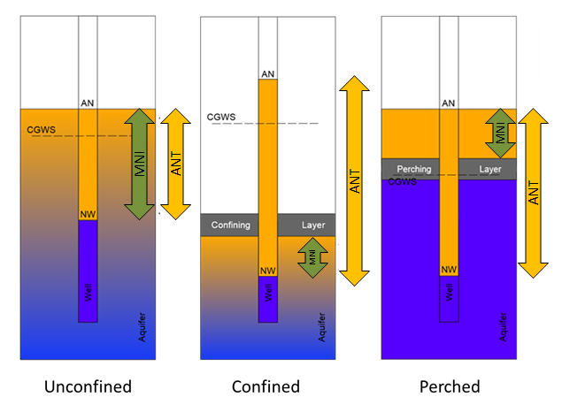
The mobile non-aqueous phase liquid (NAPL) interval (MNI) represents the thickness of the formation where NAPL is present above residual saturation. Generally this thickness can be thought of as the vertical extent corresponding to the “Shark Fin” portion of the total saturation profile. This article is the first of a two-part series on estimating the mobile NAPL interval and focuses on unconfined light NAPL (LNAPL).

Understanding the location and extent of mobile LNAPL is a critical element of the conceptual site model (CSM). Failure to understand the correct MNI will introduce error of unknown magnitude into numerical efforts to analyze and predict the distribution, mass, mobility, and recoverability of LNAPL. Quantifying the MNI is critical for calculating LNAPL drawdown under perched and confined conditions (ASTM 2013, Hawthorne 2014). Perhaps more importantly, if the MNI is unknown, then remediation efforts may target the wrong portion of the formation.

Under confined and perched LNAPL conditions, the MNI thickness and location are generally stable as the water table fluctuates because the MNI is trapped against the confining or perching layer and therefore may be vertically immobile. However, the apparent NAPL thickness (ANT) gauged in a well will change as the water table fluctuates and can be much larger than the MNI. Under unconfined conditions at equilibrium, the ANT is a good estimate of the MNI, but the MNI location and thickness may change as the water table fluctuates and the NAPL moves vertically through the formation. Consequently, it is necessary to know the LNAPL hydrogeologic condition in order to understand the MNI.

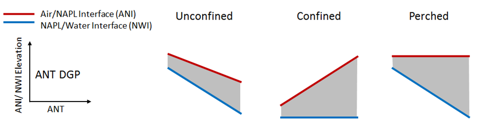
The hydrogeologic condition of the LNAPL can be identified using an ANT diagnostic gauge plot (DGP) of equilibrium gauging data (Kirkman et al, 2013; Hawthorne, 2011). Characteristic ANT DGP curves for unconfined, confined, and perched conditions are shown in Figure 2.

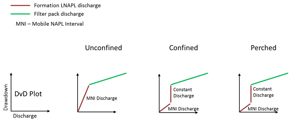
Discharge versus drawdown (DvD) plots generated from baildown tests or from gauged recharge data following manual skimming tests or oil/water ratio tests may also be used to identify the LNAPL hydrogeologic condition as well as the MNI (Kirkman et al, 2013; Hawthorne and Kirkman, 2011). Figure 3 shows characteristic DvD curves for unconfined, confined, and perched conditions.

Recognizing the characteristic patters of the DGP and DvD curves and interpreting the correct hydrogeologic condition is an important part of developing a CSM.

Unconfined Conditions
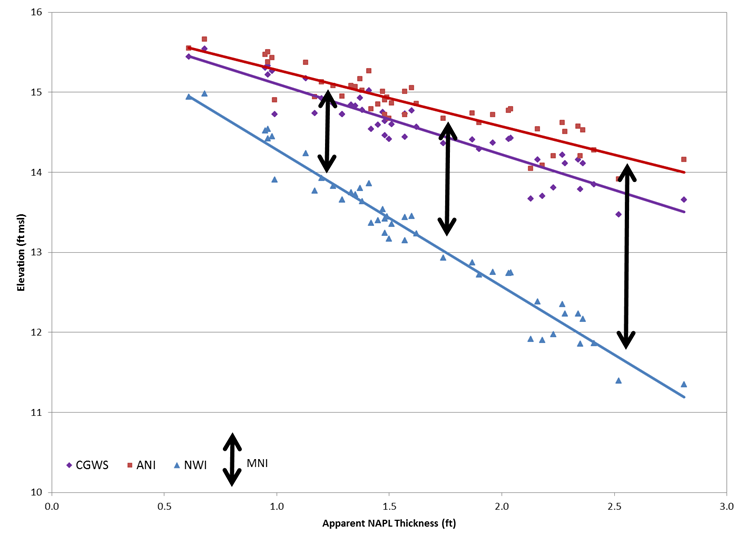
When NAPL is unconfined, the top and bottom of the MNI correspond to the ANI and NWI, respectively, and the ANT is a good estimate of the MNI. A DGP of unconfined equilibrium gauging data illustrates the range of locations and thicknesses of the MNI throughout the range of water table fluctuations (i.e., CGWS fluctuations) observed (Figure 4).

This variation in MNI occurs because as an unconfined water table rises it will typically submerge some portion of the mobile NAPL, thereby reducing the mobile NAPL saturation and thus the mobile NAPL interval. Conversely, when the unconfined water table falls, this submerged NAPL is exposed and the MNI increases.

The significance of this is that for unconfined LNAPL, some variation in LNAPL mobility, migration potential and recoverability may occur as the unconfined LNAPL and water table fluctuate up and down. Depending upon site-specific conditions, potential risk pathways, and a site-specific evaluation of the value of LNAPL recovery, this may require additional evaluation of unconfined LNAPL mobility and recoverability across the range of observed water table elevations.

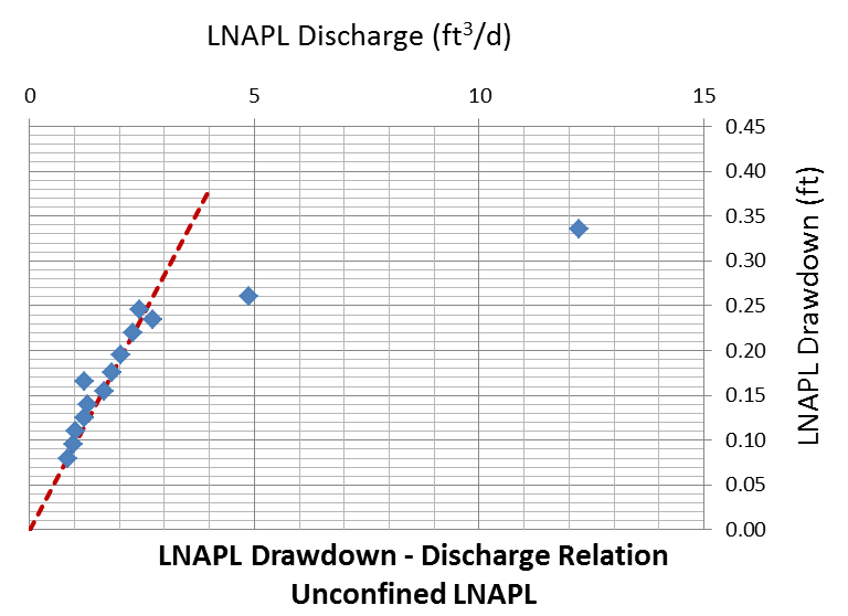
The LNAPL drawdown and the discharge rate on a DvD plot both approach zero simultaneously at equilibrium for unconfined LNAPL, as shown in Figure 5. However, the portion of the DvD plot that represents formation discharge may not represent the entire MNI due to incomplete LNAPL removal from the well and filter pack and delayed filter pack drainage that occurs across some portion of the MNI. Consequently, a DvD plot for unconfined LNAPL will often provide a lower bound on the MNI thickness, but may not identify the complete MNI. If the CGWS is at equilibrium, a lower bound MNI can be calculated by dividing the maximum observed unconfined MNI LNAPL drawdown from the DvD plot by the quantity 1 minus the NAPL/water density ratio (Kirkman et al, 2013). The upper bound is the equilibrium ANT as described above.

Summary
For unconfined LNAPL the MNI can be estimated from the apparent NAPL thickness (ANT) gauged in a well at equilibrium. Routinely bailing wells will likely result in not allowing the well to reach equilibrium conditions. This ANT and corresponding MNI represent the height of the “Shark Fin” saturation curve (i.e., the thickness of the formation with LNAPL present above residual saturation). The presence of unconfined LNAPL can be determined from DGPs and from DvD plots, and the MNI may also be estimated from DGPs, though DvDs will often not provide a complete estimate of the MNI. Identification of the MNI is critical in order to correctly calculate LNAPL mobility and recoverability, to correctly model LNAPL saturation and recovery profiles, and to correctly target the portion of the formation with recoverable LNAPL.

A Word of Caution
DGPs require equilibrium fluid data. Use of non-equilibrium data can cause inaccurate estimation of MNI. A detailed CSM is required to understand which hydrogeologic condition is appropriate and how that condition has changed, or may change, over time. Estimated MNI should be verified against other lines of evidence in the CSM. Understanding MNI is critical for calculating NAPL drawdown and transmissivity. The final results need to be interpreted within the context of the precision of the MNI estimation.

References:
ASTM
2013 Standard Guide for Estimation of LNAPL Transmissivity. ASTM E2856-13. ASTM International, West Conshohocken, PA.

Hawthorne, J. Michael
2011 Diagnostic Gauge Plots, Applied NAPL Science Review (Volume 1, Issue 2), February 2011.

Hawthorne, J. Michael
2014 Calculating NAPL Drawdown, Applied NAPL Science Review, (Volume 4, issue 3), September 2014.

Hawthorne, J. Michael, and Andrew J. Kirkman
2011 Discharge vs. Drawdown Graphs, Applied NAPL Science Review (Volume 1, Issue 4), April 2011.

Kirkman, Andrew J., Mark Adamski, and J. Michael Hawthorne
2013 Identification and Assessment of Confined and Perched LNAPL Conditions, Groundwater Monitoring & Remediation, Volume 33, Issue 1, pp 75-86.

Research Corner

Thank you to Dr. Tom Sale of the Colorado State University, Center for Contaminant Hydrology, for providing access to selected graduate level NAPL research.

Direct Measurement of LNAPL Flow in Porous Media using Tracer Dilution Techniques

Geoffrey Ryan Taylor
Master of Science
Colorado State University

Abstract: Petroleum liquids, commonly referred to as LNAPL’s, have become a basic building block of modern society. Used as fuels, lubricants, solvents and chemical feed stocks, petroleum liquids have brought many conveniences to our lives. However, a small fraction of these liquids have been inadvertently released into the subsurface forming contiguous bodies of separate phase liquids. Resolving how to manage these releases hinges largely on the rate at which these bodies are moving. To that end, a number of techniques have been developed in an effort to measure the migration, or flow rate, of LNAPL in the subsurface. Many of the current methods require challenging and costly indirect measurements to estimate this migration. The purpose of this thesis is to explore a promising new method that directly measures the flow rate of LNAPL’s, a method that builds on the tracer dilution technique used to measure the flow of groundwater. Traditional tracer dilution techniques measures the dilution of a tracer, placed into a well, to determine the flow rate of water through the well. The flow rate through the well is then used to calculate the flow rate of groundwater. The same theory applies to LNAPL’s flowing through a well. Determining the potential of the tracer dilution technique to measure LNAPL flow through a well requires investigating the mathematics governing the tracer dilution technique. A first order dilution equation was adapted for LNAPL. A method to analyze the results in a dimensionless format was also developed because it provides a technique to determine when the data conforms to the assumptions of the dilution equation. The mathematics necessary to convert the flow rate of LNAPL through a well into common measures is also derived.

Laboratory studies were conducted to verify the mathematics and to determine the applicability of the tracer dilution technique to measure LNAPL flow. At first, small scale experiments were used to visualize the dilution process and develop the technology necessary to conduct tracer dilution tests in LNAPL. A fluorescent dye, BSL 715, was selected as a tracer. A spectrometer and computer were used to measure and log the fluorescent intensity, which is a measure of the tracer concentration. A device to mix the tracer in the well without causing adverse dilution was also developed.

A large tank study explored the tracer dilution technique using a typical range of LNAPL thicknesses and flow rates. The flow rates varied from 7.2 m3/m/yr to 0.035 m3/m/yr and the LNAPL thicknesses varied from 9 cm to 24 cm. The results of the large tank study demonstrated that the tracer dilution technique is an accurate and reliable method to measure the migration of petroleum liquids in the subsurface. The measured error tends to increase at lower flow rates but is insensitive to the LNAPL thickness. The results of the large tank study led to a field test at the former ChevronTexaco Refinery in Casper, WY. The tracer dilution method was deployed in two locations. The first location was near an active recovery well where the flow rate was expected to be high. The second test was conducted in a quiescent area where the flow rate was low. The first test, near the recovery well, measured a flow rate of 0.1 m3/m/yr to 0.3 m3/m/yr. The second test, in a quiescent area, indicated a flow rate of less than 0.005 m3/m/yr. In addition, opportunities for improving sensitivity and increasing the usefulness of the method were discovered. In all, the experiments have shown the tracer dilution technique to be an effective method to directly measure the in situ migration of petroleum liquids in the subsurface.

The primary objective of ANSR is the dissemination of technical information on the science behind the characterization and remediation of Light and Dense Non-Aqueous Phase Liquids (NAPLs). Expanding on this goal, the Research Corner has been established to provide research information on advances in NAPL science from academia and similar research institutions. Each issue will provide a brief synopsis of a research topic and link to the thesis/dissertation/report, wherever available.

Practical Stats

Top Twelve Tip #6:
Understand assumptions behind the methods

Dr. Dennis Helsel
www.practicalstats.com

Correlation is seen as answering a general question – “Is there a systematic relation between these two variables?” The most commonly used correlation coefficient is Pearson’s r. Pearson’s coefficient should be remembered as “Pearson’s LINEAR correlation coefficient”. It measures the strength of a LINEAR association between two variables. There are other types of correlation, and correlation coefficients. The graph on the left below shows two variables generated to have a linear relationship. In addition to Pearson’s r, Spearman’s rho and Kendall’s tau also measure correlation — monotonic (heading in the same direction, but not necessarily at a constant rate) correlation. All three coefficients do an outstanding job of seeing the linear correlation in the left graph below. Note: Kendall’s tau is measured on an alternate scale approximately 0.15 to 0.20 below the others two coefficients for the same strength of correlation (like Centigrade vs Fahrenheit).

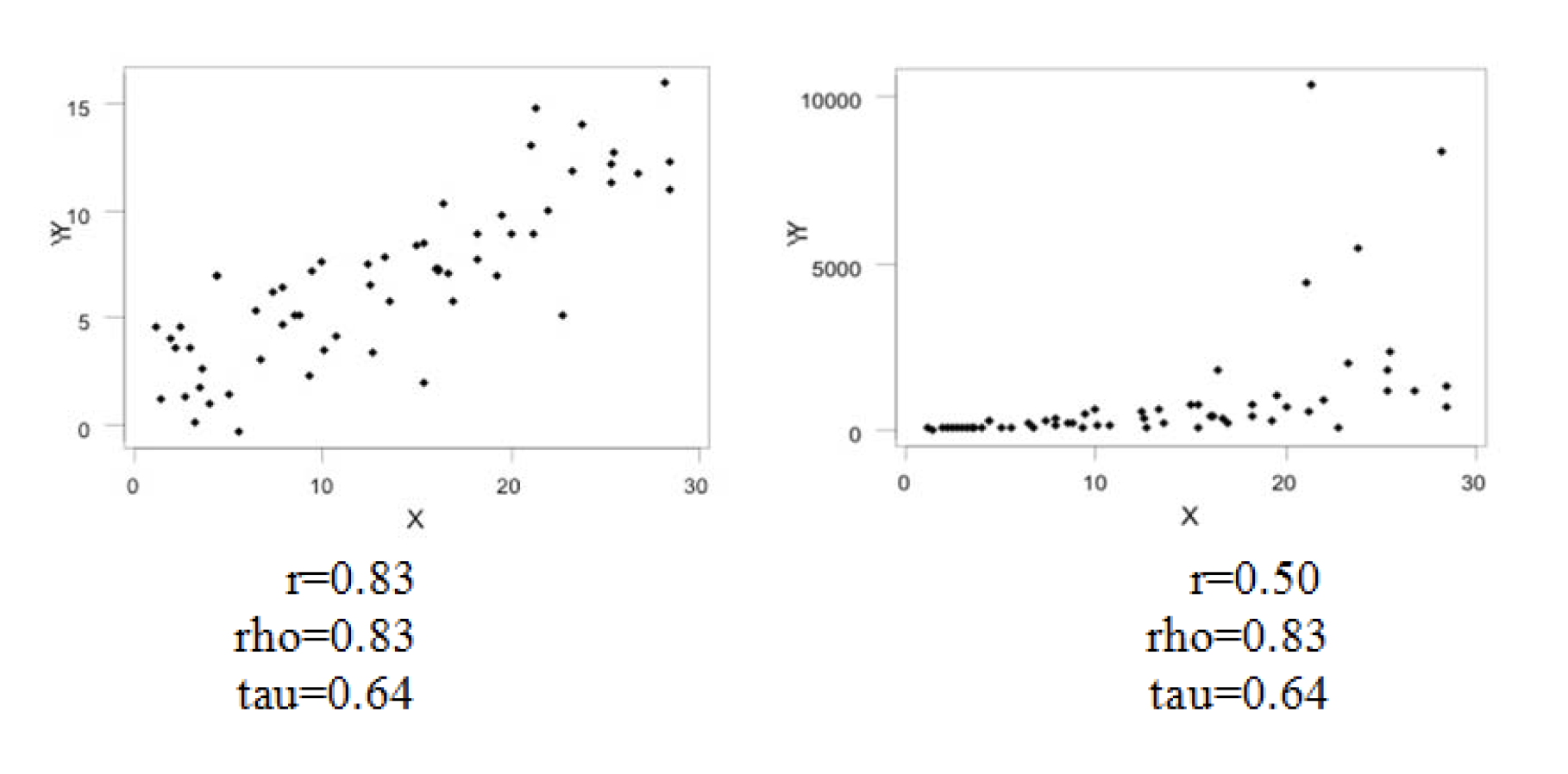
Now look to the right. The Y variable was cubed to produce a nonlinear relation — the slope between Y and X now changes as X increases. Pearson’s r (0.50) cannot see the relation as well because the pattern is not linear. Rho and tau remain exactly the same because the order of observations stays the same. Rho and tau are not dependent on a linear model of the relationship. They measure both linear and nonlinear correlation.

Make sure that you understand the assumptions of the methods you use, and use the tool that best fits your objective. If you want a general measure of “systematic relation,” rho or tau would be more appropriate than Pearson’s r. Kendall’s tau is commonly used in trend analysis as a flexible measure of change versus time. Do you really want to only look for linear patterns?