Rate Transient Analysis and Modeling Future Performance
Volume 7, Issue 1 | April 2017

Applied NAPL Science Review

Demystifying NAPL Science for the Remediation Manager

Editor: J. Michael Hawthorne, PG

ANSR Scientific Advisory Board
J. Michael Hawthorne, PG, Board Chairman, GEI Consultants, Inc
Mark Adamski, PG, Statoil
Stephen S. Boynton, PE, LSP, Subsurface Env. Solutions, LLC
Dr. Randall Charbeneau, PE, University of Texas
Paul Cho, PG, CA Regional Water Quality Control Board-LA
Robert Frank, RG, CH2M
Dr. Sanjay Garg, Shell Global Solutions (US) Inc.
Randy St. Germain, Dakota Technologies, Inc.
Dr. Dennis Helsel, Practical Stats
Dr. Terrence Johnson, USEPA
Andrew J. Kirkman, PE, BP Americas
Mark Lyverse, PG, Chevron Energy Technology Company
Mark W. Malander, ExxonMobil Environmental Services

Applied NAPL Science Review (ANSR) is a scientific ejournal that provides insight into the science behind the characterization and remediation of Non-Aqueous Phase Liquids (NAPLs) using plain English. We welcome feedback, suggestions for future topics, questions, and recommended links to NAPL resources. All submittals should be sent to the editor.

DISCLAIMER: This article was prepared by the author(s) in their personal capacity. The opinions expressed in this article are the author’s own and do not necessarily reflect the views of Applied NAPL Science Review (ANSR) or of the ANSR Review Board members.

Decline curves are one component of a comprehensive strategy to effectively demonstrate attainment of a sound technology decision point that incorporates cumulative decline curves, expected ultimate recovery decline curves, rate-transient analysis decline curves, LNAPL transmissivity calculations, modeling of recoveries and saturations using the LNAPL Distribution and Recovery Model, and incorporation of the ITRC proposed LNAPL transmissivity endpoint range. This article is the second in a series that will address these topics for the hydraulic recovery of LNAPL.

Rate Transient Analysis and
Modeling Future Performance

Rate Transient Analysis
Rate transient analysis (RTA) is a tool to estimate the time required to reach recovery thresholds for non-aqueous phase liquid (NAPL) recovery systems. It provides a quantitative approach to represent de minimis recovery thresholds used to determine when recovery systems can be shut down, such as “diminishing returns” or “asymptotic recovery.”

This article provides a brief introduction to the analysis method and is not intended to cover all of the considerations required for variables that can affect the quality of the fit. The methodologies presented are focused on isotropic mediums where the recovery rate is primarily being affected by the remaining mass. A robust conceptual site model (CSM) is required to verify that other environmental variables (e.g., fluctuating water table or a migrating plume) and/or operational changes (e.g., extended downtime) are not affecting the analysis or are corrected for. These evaluations and adjustments may be topics for future ANSR articles (see Sale 2001 and Poston and Poe 2008 for a more detailed discussion of RTA methodologies and assumptions).

RTA analysis is performed by constructing a semi-log, rate-time decline curve where the elapsed time is plotted on the x-axis and the logarithm of recovery rate is plotted on the y-axis (Poston and Poe 2008, Sale 2001). Most commonly, the recovery rate is decreasing exponentially with time in remediation applications, and the data will exhibit a semi-log linear trend, as shown in Figure 1. If the rate-time data does not decrease exponentially, the recovery rate may be decreasing linearly, hyperbolically, or harmonically with time (see Poston and Poe 2008 for more on analysis of non-exponential decline curves).

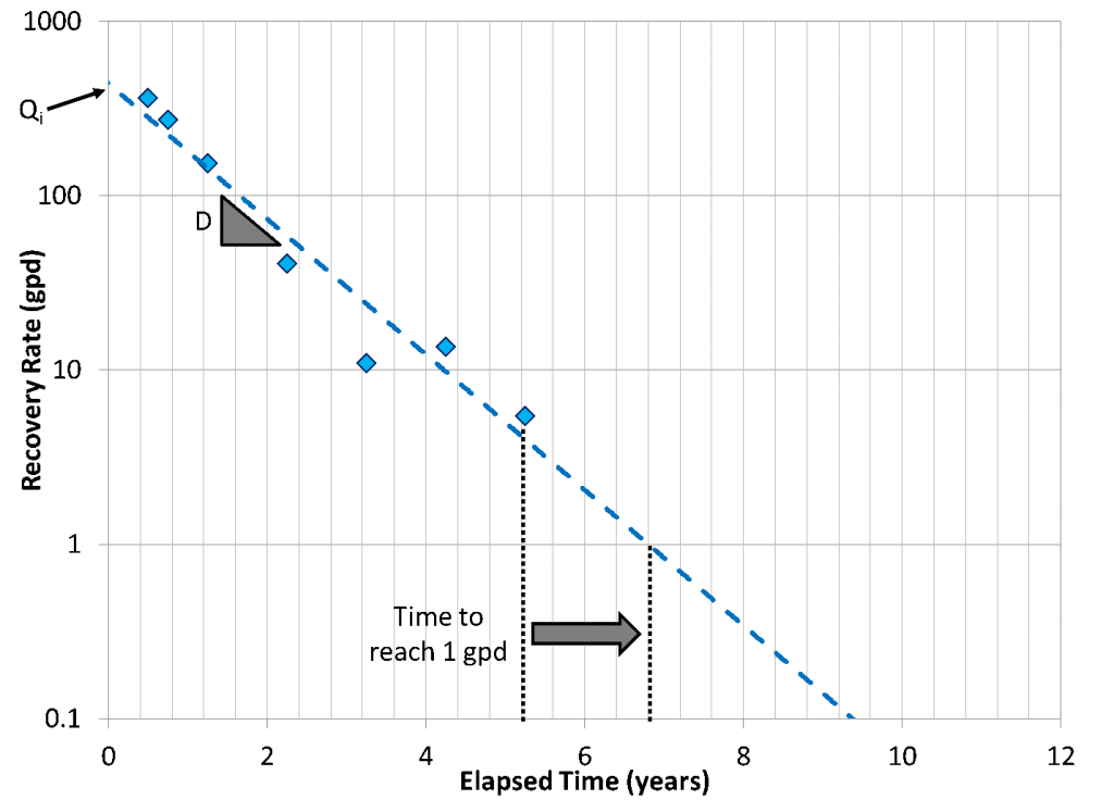
The data is fit to a line of the form:

where Q is the modeled recovery rate [L³/T], Qi is the calculated initial recovery rate [L³/T], and D is the decline rate [1/T] (the slope of the fitted line). The initial recovery rate (Q_i) is the intercept of the fitted line, which is the recovery rate predicted by the curve fit, not the initial measured value.

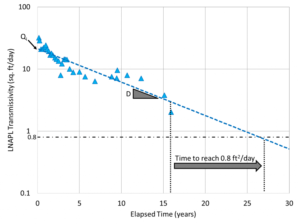
RTA charts can also be constructed using light non-aqueous phase liquid (LNAPL) transmissivity in place of LNAPL recovery, as shown in Figure 2. This approach is beneficial to track progress towards an LNAPL transmissivity threshold metric. Using LNAPL transmissivity for the decline curve may also normalize variations in operability, often resulting in a more accurate analysis than recovery rate alone.

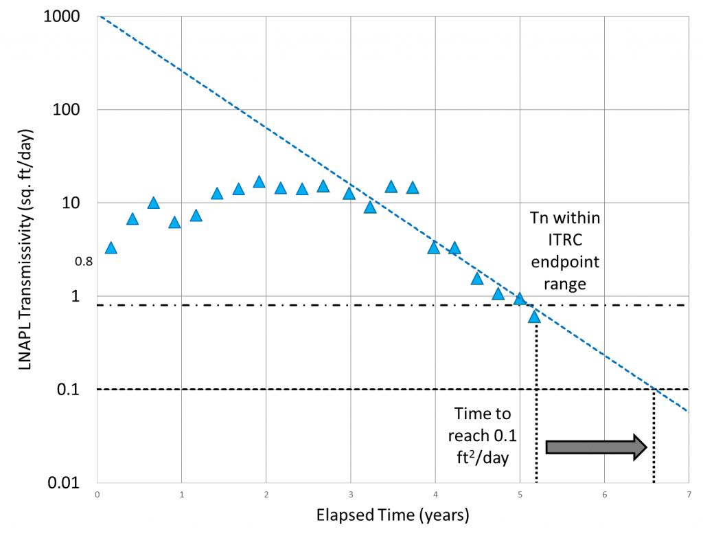
Frequently, the decline rate will change over time. When hydraulic recovery begins, it takes some time to establish constant boundary conditions around the well. The LNAPL recovery rate may increase for a period of time, as the LNAPL redistributes towards the well, and then decrease. Changes in environmental conditions (e.g., fluctuating water table or a migrating plume) and/or operational changes (e.g., extended downtime) may affect the projections. Having a robust CSM is therefore critical in helping to understand these potential projection estimate changes and the degree to which the projections may be affected. The data used for the projection should be representative of the reasonably anticipated future conditions, and the line should be fit only to the late time data with a constant slope as shown in Figure 3.

Modeling with RTAs
RTA can be utilized to predict the remaining time to reach a de minimis or regulatory threshold. For example, Figure 1 illustrates projection to a site specific recovery rate threshold, such as 1 gallon per day. Another common example (Figure 2) is based on a threshold LNAPL transmissivity, such as 0.8 foot squared per day (ft²/day), which can be used to represent achievement of recovery of LNAPL to the maximum extent practical in states that accept that threshold (e.g., Massachusetts, MassDEP 2016; Kansas, KDHP 2015). Where the regulatory environment is less prescribed, the RTA can be compared to the range of 0.1 to 0.8 ft²/day proposed by the ITRC (ITRC 2009), as shown in Figure 3.

Another potential approach is to combine the RTA with an Expected Ultimate Recovery (EUR) analysis. The EUR volume represents the theoretical maximum volume of NAPL that can be produced from a hydraulic recovery well given infinite time. The methodology to estimate the EUR volume was presented in “Estimating Expected Ultimate Recovery” (Reyenga, 2016). The time required to reach a given threshold (e.g., 90 percent of the EUR volume) can be estimated by combining the curve fits from both RTA and EUR analyses.

Each of these can be a powerful tool for site management as well as to provide quantitative lines of evidence for when hydraulic recovery is no longer effective.

A Word of Caution
Decline curves require accurate estimation of the volumes and rates of LNAPL recovery. Particular attention must be paid to the estimation of LNAPL volume as it decreases to the limit of measurement. Inconsistent assessment of the volumes associated with an LNAPL sheen, foam, meniscus, or emulsion in the field or the office can have a significant effect on the estimated volume of LNAPL recovered. In some cases, LNAPL transmissivity may be able to provide an accurate decline curve, when recovery rates cannot, by normalizing changes in conditions over time. A thorough understanding of the site conceptual model is also required to ensure the decline observed is due to successful reductions in saturations in the subsurface rather than changes in field condition (such as water table elevation) and/or operational inefficiencies, and that the conditions during the period of constant decline are representative of reasonably anticipated future conditions.

References:
Commonwealth of Massachusetts Department of Environmental Protection (MassDEP 2016)
2016 Light Nonaqueous Phase Liquids (LNAPL) and the MCP: Guidance for Site Assessment
and Closure. February 2016.

The Interstate Technology & Regulatory Council (ITRC)
2009 Evaluating LNAPL Remedial Technologies for Achieving Project Goals.
December 2009.

Kansas Department of Health and Environment (KDHP 2015)
2016 Total Petroleum Hydrocarbons (TPH) and Light Non-Aqueous Phase Liquid (LNAPL)
Characterization, Remediation and Management. September 2015.

Poston, Stephen W. and Bobby D. Poe
2008 Analysis of Production Decline Curves. Society of Petroleum Engineers, 2008.

Reyenga, Lisa
2016 Estimating Expected Ultimate Recovery. Applied NAPL Science Review Volume 6
Issue 2, July 2016.

Sale, Tom
2001 Methods for Determining Inputs to Environmental Petroleum Hydrocarbon Mobility and
Recovery Models. American Petroleum Institute Publication Number 4711, July 2001.

Research Corner

Thank you to Dr. Tom Sale of the Colorado State University, Center for Contaminant Hydrology, for providing access to selected graduate level NAPL research.

LNAPL longevity as a function of remedial actions : tools for evaluating LNAPL remedies

Anna Meryle Skinner
Master of Science
Colorado State University

Abstract:
The impacts of remedial measures on the longevity of light non-aqueous phase liquid [LNAPL] releases are rarely quantified at sites where active remediation of LNAPL bodies has been carried out. Without an understanding of LNAPL longevity, decisions regarding the appropriateness of remediation strategies and their scheduling in the life cycle of an LNAPL release could be regarded as arbitrary in some respects. Because LNAPL bodies are continually evolving with respect to composition, internal and external transport, distribution, and lateral and longitudinal mobility, it appears that a necessary part of any site conceptual model guiding remediation decisions should include an understanding of LNAPL evolution over time in terms of mass remaining. Understanding LNAPL remaining versus time would enable decision makers to estimate and compare the effects of various treatment remedies, combinations thereof, and different scheduling of treatment remedies within the remedial time frame. This thesis presents work done to develop a novel LNAPL longevity predictive model [LLPM]. A series of laboratory sand tank experiments were conducted to gain an improved understanding of the effects of natural losses and remedial measures on LNAPL longevity as well as provide laboratory-scale input parameters for the development of the LLPM.

Results from the laboratory studies were then used as a basis for developing and testing the LLPM. The laboratory work consisted of four sand tank experiments in which a known mass of LNAPL was introduced to the system. Measurements were taken throughout the expansion and depletion of the LNAPL pool to track remaining LNAPL. These measurements were used to describe the evolution of the LNAPL releases over the experimental time frame. Different remediation approaches were applied to each experiment to determine their effects on LNAPL release evolution and overall longevity. The two treatment remedies that were applied were LNAPL recovery via well skimming and water table fluctuations. A base scenario was established by not applying either remedy. Next, one experiment was conducted where each of the treatment remedies was applied singly. The final experiment was conducted by applying both treatment remedies. Methyl-tert-butyl ether [MTBE] was the LNAPL used in the laboratory experiments. The experimental data showed that LNAPL recovery decreased the longevity of the MTBE release, while water table fluctuations acted to increase longevity. The increase caused by water table fluctuations was smaller than the decrease caused by LNAPL recovery. Mass balance measurements from laboratory experimentation were used to develop a version of the model that could be tested with laboratory-scale data.

A key result was that LNAPL can be fully depleted over time by natural and/or engineered processes. The LLPM was then developed by applying numerical methods to combinations of zero and first order ordinary differential equations used to simulate LNAPL depletion processes. Laboratory-scale input parameters were used to test the LLPM against data from the laboratory experiments. A field-scale application and sensitivity analysis of the LLPM were completed to demonstrate the field-scale capabilities of the model and examine which governing processes had the greatest effects on LNAPL longevity and evolution. One significant difference was recognized between the laboratory-scale and field-scale input. In the laboratory experiments, the dominant loss mechanism was volatilization, while in the field, biological degradation is thought to be most significant.

First, the model was developed by combining numerical solutions for zero and first order reaction rate differential equations. First order loss rates change as the mass in the system changes, whereas zero order loss rates are constant regardless of how much mass remains in the system. Based on available literature, volatilization, dissolution, and biological degradation were modeled as zero order processes, while active remedies such as LNAPL/hydraulic recovery and Soil Vapor Extraction were modeled as first order processes. Loss mechanisms were applied to the LNAPL release according to the distribution of mass between two compartments: one containing the continuous fraction of LNAPL and the other containing the discontinuous fraction.

Another important parameter that became apparent through the literature review was subsurface temperature. The rate at which biological degradation occurs was found to be related to temperature; therefore, fluctuations in temperature can produce corresponding fluctuations in the overall depletion rate of LNAPL. Next, the accuracy of the model was tested using mass balance data from the laboratory experiments. Simulations of the sand tank experiments with laboratory-scale data achieved a favorable fit between the model and experimental data. This signaled that the model was ready to be applied to a field-scale scenario. Field-scale input parameters were used to demonstrate the field -scale application and conduct a sensitivity analysis of the LLPM. The sensitivity analysis examined the relative effects of two treatment remedies: hydraulic recovery and thermal enhancement of biological degradation. This analysis showed that the mass distribution of LNAPL between the two designated fractions plays an important role in the evolution of the LNAPL release and the effectiveness of remediation technologies.

It was also concluded that all parameters related to hydraulic recovery had a significant impact on the LNAPL longevity and evolution. For example, the effectiveness of hydraulic recovery to reduce LNAPL longevity was reduced as hydraulic recovery was scheduled later in the release time frame. Therefore, the life cycle stage of a LNAPL release may play a role in the effectiveness and appropriateness of various treatment remedies. The results of the laboratory sand tank experiments also support this idea. This suggests the evaluation of the interactions of multiple remedies and natural losses will be necessary to develop an accurate analysis of LNAPL longevity and evolution as LNAPL releases pass through different life cycle stages.

The effects of water table fluctuations on LNAPL mass distribution, longevity, and evolution were examined. Because different loss mechanisms affect LNAPL in the different fraction compartments, the effects of water table fluctuations were thought to be important. Water table fluctuations act to distribute LNAPL mass vertically throughout a smear zone. This may produce averaging effects that support the designation of biological degradation as a zero order process. The beta version of the LLPM developed herein has specific limitations and challenges. One of the most significant challenges of this work is a lack of field-scale LNAPL longevity and evolution data to compare to the results of the LLPM. Suggestions for future work to address these limitations and challenges are given. One example is that of conducting multi-component LNAPL laboratory sand tank studies. These types of studies would further develop the conceptual model of LNAPL releases and increase the field applicability of the LLPM to real world sites where multi-component contaminants are often present. Future work should be done to make the model more robust and derive next generation versions of the LLPM. Through future work it is anticipated that a version of the LLPM will be developed that practitioners can use to guide sustainable remediation planning for LNAPL sites.

The primary objective of ANSR is the dissemination of technical information on the science behind the characterization and remediation of Light and Dense Non-Aqueous Phase Liquids (NAPLs). Expanding on this goal, the Research Corner has been established to provide research information on advances in NAPL science from academia and similar research institutions. Each issue will provide a brief synopsis of a research topic and link to the thesis/dissertation/report, wherever available.

Practical Stats

Top Twelve Tip #10:
Know Your Target for Trend Analysis

Trend analysis is any test where one of the explanatory (x) variables is time. Continuous trends are often measured using linear regression or the Theil-Sen line (the line that goes with the “Mann-Kendall test for trend”). Step trends are tested using two group tests (the t-test or Wilcoxon rank-sum tests) comparing conditions before vs. after a specific date or event.

What is a trend? In statistics, a trend is monotonic — it goes in predominantly one direction, an overall increase or decrease. Patterns that go up and then down again are technically not trends, even though they can be modeled with polynomial regressions or other techniques. One of the important cyclical (non-trend) patterns in environmental systems is seasonality, the tendency at one time of year for values to be higher than average, and at another time of the year to be lower.

Parametric trend analysis incorporates seasonality by building a more complex regression model. Sine and cosine terms are added to the regression equation where time is the explanatory (x) variable. Sine and cosine model a wave pattern that is fit to the pattern of the data, peaking at the time of year observed at the site. This provides better predictions, as well as removing noise in order to see the trend more clearly (see Tip #7). Nonparametric trend analysis (usually methods based on Kendall’s tau correlation) split up the data into seasonal “blocks”, performing the test separately on each block and combining the results into one overall test. No comparisons across seasons are made — no comparison is made of June data in later years to January data in earlier years, etc.

The most prevalent trend test in environmental studies is a nonparametric test with blocking, the Seasonal Kendall test, developed at the US Geological Survey by Hirsch and others in the 1980s. Computed on the original data, it tests whether values are increasing, decreasing, or staying the same. Just as commonly, the trend test is computed on data adjusted for a covariate such as depth to water or another possible cause of change. By adjusting for or ‘factoring out’ that other variable, the test focuses on the targeted cause of the trend. This again utilizes Tip #7 (see www.practicalstats.com/top12tips/), factoring out the ‘noise’ due to changing (often natural) influences to focus on trends due to variables (human effects) that might be able to be managed. For more information on trend analysis, see the chapter in the free textbook Statistical Methods in Water Resources by Helsel and Hirsch, available as book #2 at www.practicalstats.com/books/.