Applied NAPL Science Review
Demystifying NAPL Science for the Remediation Manager
Editor: J. Michael Hawthorne, PG
Asst. Editor: Dr. Rangaramanujam Muthu
ANSR Scientific Review Board
J. Michael Hawthorne, PG, Board of Chairman, GEI Consultants Inc.
Mark Adamski, PG, BP Americas
Stephen S. Boynton, PE, LSP, Subsurface Env. Solutions, LLC
Dr. Randall Charbeneau, University of Texas
Paul Cho, PG, CA Regional Water Quality Control Board-LA
Dr. Sanjay Garg, Shell Global Solutions (US) Inc.
Dr. Terrence Johnson, USEPA
Andrew J. Kirkman, PE, BP Americas
Mark Lyverse, PG, Chevron Energy Technology Company
Mark W. Malander, ExxonMobil Environmental Services
Applied NAPL Science Review (ANSR) is a scientific ejournal that provides insight into the science behind the characterization and remediation of Non-Aqueous Phase Liquids (NAPLs) using plain English. We welcome feedback, suggestions for future topics, questions, and recommended links to NAPL resources. All submittals should be sent to the editor.
LNAPL Body Stability
Part 2: Daughter Plume Stability
via Spatial Moments Analysis
GEI Consultants, Inc. and Practical Stats
Editors Note: Due to the variety and potential complexity of all of the potential lines of evidence to evaluate for LNAPL body stability, this is the first in a series of articles providing examples of how to evaluate LNAPL body stability.
In ANSR volume 3 issue 4, LNAPL Body Stability, we discussed the various lines of evidence applicable to LNAPL body stability. In this issue we will discuss spatial moments analysis, which is one type of analysis that can be used to evaluate dissolved-phase stability. Spatial moments analysis may be conducted formally (MAROS, 2006; MAROS, 2012) or informally (Ricker, 2008).
Three spatial mass moments may be evaluated:
- Zeroith Moment: Estimated Total Plume Mass
- First Moment: Center of Plume Mass (relative to source location)
- Second Moment: Distribution of Plume Mass (relative to source location)
The objective for spatial moments analysis is to determine what the spatial trends over time are for the dissolved-phase plume. A stable dissolved-phase plume is typically a robust indicator of the overall NAPL body stability. Basically we’re trying to determine if the dissolved-phase plume (and by extension the NAPL body) is stable by determining if:
- The total dissolved-phase mass is stable to decreasing,
- the center of that mass is stable or retreating, and
- the overall distribution of the dissolved-phase mass is stable.
MAROS (2006; 2012) contains a formalized spatial moments analysis procedure, and subsequent statistical analyses based on the nonparametric Mann-Kendall test to identify trends in the data from which plume stability may be interpreted. Ricker (2008) describes an informal spatial moments analysis method utilizing Surfer™ and Excel™, with linear regression to determine trends. MAROS provides a more rigorous statistical evaluation of both individual well and holistic plume stability. The Ricker method tends to be more intuitively transparent and focuses on a holistic plume evaluation. Both methods provide meaningful evaluations of plume stability.
Once spatial moments have been calculated, they may be mapped or graphed for visual demonstration and analysis. For example, the zeroith moment (mass estimate over time) may be graphed (Figure 1) and analyzed statistically to determine if a trend exists. A decreasing trend suggests that mass contributions from the plume source may have decreased or stopped. An increasing trend suggests that existing or new source contributions continue to occur. A stable trend suggests that the plume is in steady state relative to potential mass contributions and natural attenuation.
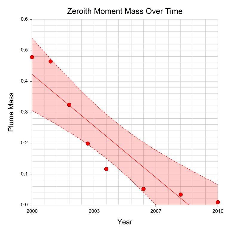
Figure 1. Time series graph of zeroith moment data (plume mass) with a regression line and 95% confidence limits shown (MAROS, 2012).
A time-series analysis of the first mass moment (change of location of center of mass) may be plotted on a map or converted to downgradient distance from some location (e.g., source) and plotted on a graph (Figures 2 and 3). Trends in center of mass location over time often track plume migration trends (e.g., if the center of mass is retreating towards the source area then the plume may be shrinking).
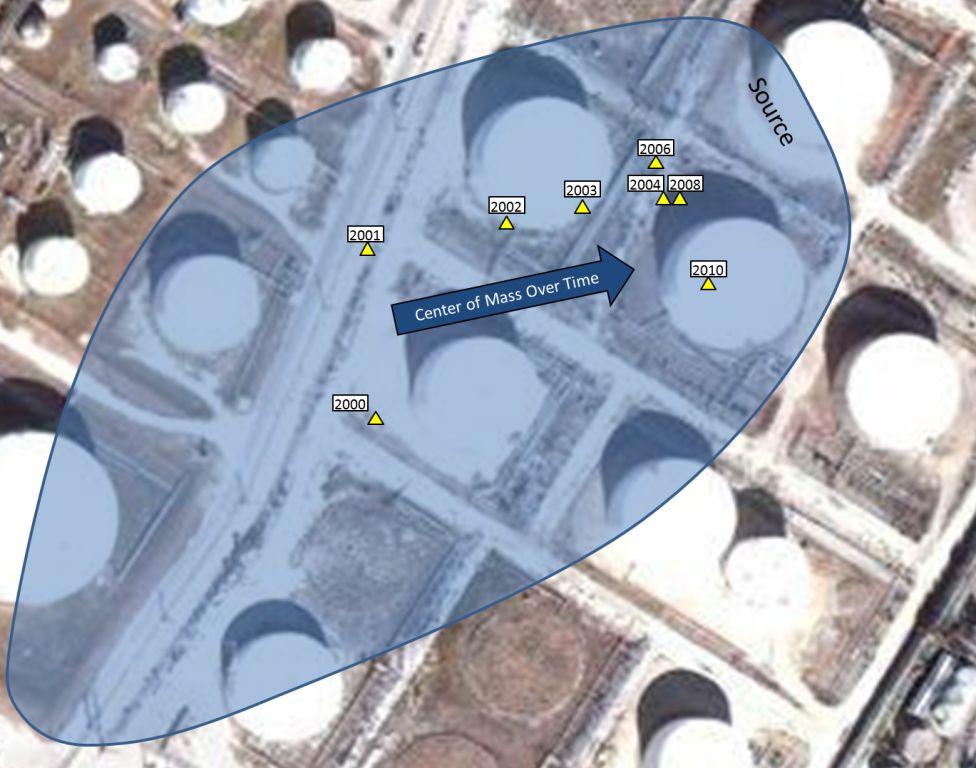
Figure 2. Hypothetical depiction of first moment center of mass movement towards source area of an overall plume footprint over time due to attenuation of plume mass.
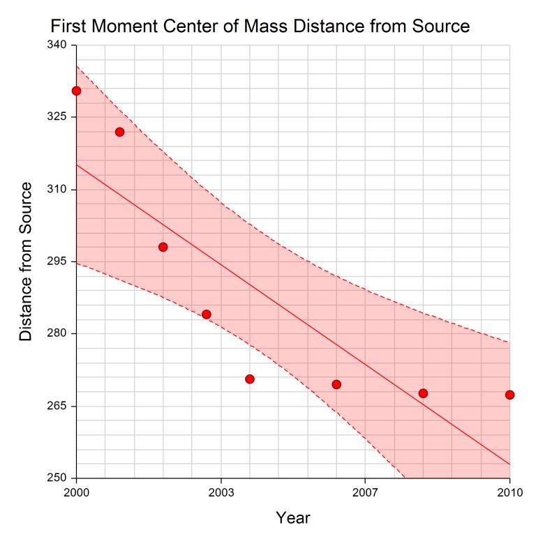
Figure 3. First moment distance from source to center of mass over time with a regression line and 95% confidence limits shown (MAROS, 2012).
The second mass moment provides an estimate of the plume mass spatial distribution about the center of mass. Time-series analysis of the second mass moment is useful for demonstrating re-distribution of mass within the plume over time, which reflects plume footprint expansion or contraction (e.g., If the distribution of plume mass becomes increasingly distant from the center of mass, the plume footprint may be interpreted to be expanding).
Any interpretation of the spatial moments analysis must account for all moments. For example, a second moment trend away from the plume center of mass might suggest the plume is expanding. However, if during the same time the zeroith moment indicates an overall decreasing plume mass, the data would be consistent with a plume whose core is being attenuated more rapidly than its margin.
Trend tests such as Mann-Kendall which are based on Kendall’s tau correlation are widely-used in field studies because they have few prerequisites (e.g., data do not have to follow a normal distribution, nondetect values can be incorporated). If the Mann-Kendall tests for the first or second moment data indicate a significant trend (see this month’s Practical Stats column), the slope of that trend estimates the median or typical rate of change in the moment, determining the speed at which conditions are changing. If multiple sites have sufficient data to be tested for trend, those tests can be combined into one overall evaluation using the Regional Kendall test (see ANSR v3i4). The Regional Kendall test evaluates whether a consistent change takes place across multiple sites within the larger study area.
A word of caution is in order with respect to spatial moments analysis. If the same wells are sampled in each event, then the calculated spatial moments will be faithful reflections of the dissolved-phase body over time (within achieved error limits for field sampling and laboratory analysis). However, if different wells are sampled over time, then variation in the calculated moments may be a result of either actual variations in the mass moments over time or variation in the wells sampled over time or both. Before blindly accepting a numerical, graphical, or statistical trend analysis result, make sure that you understand the limitations of the data set. Remember that although daughter phase body stability is a powerful indicator of LNAPL body stability (i.e., if the dissolved-phase constituents are stable, then by indirect evaluation, the LNAPL must also be stable), spatial moments analysis of daughter phase body stability is only one particular type of analysis for one line of evidence for LNAPL body stability. Additional lines of evidence should typically be examined to ensure a clear understanding of LNAPL body stability issues for the site or release.
References:
MAROS (2006, 2012) Monitoring and Remediation Optimization System (MAROS) User’s Guide and Technical Manual, developed by GSI Environmental, Inc. for the Air Force Center for Engineering and the Environment, 98 pp.
Ricker, Joseph A. (2008) A Practical Method to Evaluate Ground Water Contaminant Plume Stability, Groundwater Monitoring & Remediation, volume 28, no. 4, Fall, pp 85-94.
Practical StatsDr. Dennis Helsel The Mann-Kendall test for trend is the most widely used trend test in water quality and other environmental disciplines. It tests for whether there is a significant trend over time, even if that trend is not linear. The test is a simple correlation coefficient, Kendall’s tau, when one of the two variables is time. If there is a correlation with time, there is by definition a trend. Figure 1 Figure 1 shows the six measurements of transmissivity in well 5 from data from ANSR volume 3, issue 4. Kendall’s tau is computed by determining if there are consistent increases or decreases when comparing all observations to one another. If no trend exists, half increases and half decreases would be expected just from random data variation. Comparison of the 2007 observation to later measurements shows four increases (+) and one tie (0). All comparisons after 2007 increase with time. Out of the 15 comparisons, 14 are increases and 1 is a tie. There were no decreases. The probability of getting 14 out of 15 increases when only 7 or 8 (15 divided by 2) are expected by chance seems small. The p-value, which is the probability of getting 14 (or even more) increases out of the 15 comparisons in time sequence, answers the question “what is the probability of getting this result just by accident?” It turns out to be 0.013 – a consistent increase like this would occur only 13 out of 1,000 times when there really was no trend. Such a small probability causes the scientist to state that a significant trend is indicated. Note that no restrictive assumptions about the shape of the data or the rate of increase were needed (this is a nonparametric test). If we want a measurement of the rate of change, Figure 1 shows that this rate is not constant – the increase is curved. To use a straight line equation (i.e., a constant slope), we can transform the data by taking cube roots. Data in the resulting graph (Figure 2) look linear, and the equation of the significant Mann-Kendall (blue) line is cube root of transmissivity = -454.4 +0.226 * Year which can be re-transformed back into units of transmissivity. Note that the test itself remains the same regardless of whether the data are transformed or not. Figure 2 For more information on trend tests and other statistical methods for practical use, attend our Applied Environmental Statistics course this November. Details are at |


Related Links
API LNAPL Resources
ASTM LCSM Guide
Env Canada Oil Properties DB
EPA NAPL Guidance
ITRC LNAPL Resources
ITRC LNAPL Training
ITRC DNAPL Documents
RTDF NAPL Training
RTDF NAPL Publications
USGS LNAPL Facts
ANSR Archives
Coming Up
Look for more articles on LNAPL transmissivity as well as additional explanations of laser induced fluorescence, natural source zone depletion and LNAPL Distribution and Recovery Modeling in coming newsletters.
Announcements
An updated version of the ASTM Guide for Calculating LNAPL Transmissivity is Now Available for Purchase at www.astm.org.
ASTM Standard E2856 – Standard guide for Estimation of LNAPL Transmissivity is now available
The ASTM LNAPL Conceptual Site Model (LCSM) workgroup is actively updating the ASTM LCSM guidance document. If you are interested in participating on this team or would like to send comments for consideration – please contact Andrew Kirkman of BP Americas (team leader).
ANSR now has a companion group on LinkedIn that is open to all and is intended to provide a forum for the exchange of questions and information about NAPL science. You are all invited to join by clicking here OR search for “ANSR – Applied NAPL Science Review” on LinkedIn. If you have a question or want to share information on applied NAPL science, then the ANSR LinkedIn group is an excellent forum to reach out to others internationally.