Estimating Expected Ultimate Recovery
Volume 6, Issue 2 | July 2016

Applied NAPL Science Review

Demystifying NAPL Science for the Remediation Manager

Editor: J. Michael Hawthorne, PG

ANSR Scientific Advisory Board
J. Michael Hawthorne, PG, Board Chairman, GEI Consultants, Inc
Mark Adamski, PG, Statoil
Stephen S. Boynton, PE, LSP, Subsurface Env. Solutions, LLC
Dr. Randall Charbeneau, PE, University of Texas
Paul Cho, PG, CA Regional Water Quality Control Board-LA
Robert Frank, RG, CH2M
Dr. Sanjay Garg, Shell Global Solutions (US) Inc.
Randy St. Germain, Dakota Technologies, Inc.
Dr. Dennis Helsel, Practical Stats
Dr. Terrence Johnson, USEPA
Andrew J. Kirkman, PE, BP Americas
Mark Lyverse, PG, Chevron Energy Technology Company
Mark W. Malander, ExxonMobil Environmental Services

Applied NAPL Science Review (ANSR) is a scientific ejournal that provides insight into the science behind the characterization and remediation of Non-Aqueous Phase Liquids (NAPLs) using plain English. We welcome feedback, suggestions for future topics, questions, and recommended links to NAPL resources. All submittals should be sent to the editor.

DISCLAIMER: This article was prepared by the author(s) in their personal capacity. The opinions expressed in this article are the author’s own and do not necessarily reflect the views of Applied NAPL Science Review (ANSR) or of the ANSR Review Board members.

Decline curves are one component of a comprehensive strategy to effectively demonstrate attainment of a sound technology decision point that incorporates cumulative decline curves, expected ultimate recovery decline curves, rate-transient analysis decline curves, LNAPL transmissivity calculations, modeling of recoveries and saturations using the LNAPL Distribution and Recovery Model, and incorporation of the ITRC proposed LNAPL transmissivity endpoint range. This article is the first in a series that will address these topics for the hydraulic recovery of LNAPL.

Estimating Expected Ultimate Recovery

Expected Ultimate Recovery
The expected ultimate recovery (EUR) is the theoretical maximum volume of non-aqueous phase liquid (NAPL) that can be produced from a hydraulic recovery well. Estimating the EUR provides a powerful tool to evaluate the effectiveness of recovery operations and to estimate the time required to reach critical recovery thresholds.

The EUR is estimated by constructing a rate-cumulative decline curve where the cumulative recovered volume is plotted on the x-axis and the recovery rate is plotted on the y-axis (Poston and Poe 2008, Sale 2001). Most commonly in remediation applications, the data will exhibit a linear trend, as shown in Figure 1. This case corresponds to conditions where the recovery rate is decreasing exponentially with time. If the rate-cumulative data does not decrease linearly, the recovery rate may be decreasing linearly, hyperbolically, or harmonically with time. For more information on analyzing non-linear rate-cumulative decline curves see Analysis of Production Decline Curves (Poston and Poe 2008).

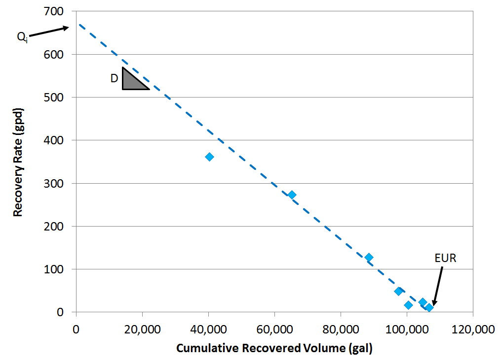
The EUR is estimated by fitting a line through the data and projecting it to intersect the x-axis. This point represents the maximum potential volume of light non-aqueous phase liquid (LNAPL) that could be removed from the well given infinite time when the recovery rate reaches zero. However, in practice the recovery rate typically falls below a de minimis threshold where hydraulic recovery is no longer practical prior to achieving the full EUR volume.

The EUR is calculated as:

Where Qi is the calculated initial recovery rate [L³] and D is the decline rate [1/T]. Note that the initial recovery rate is the value predicted by the curve fit (where it crosses the y-axis), not the initial measured value. It is not recommended to make projections based on initial measured values until a constant decline rate is established (see below). If a commercial program is used to fit the data into a “y = mx + b” format, the decline rate corresponds to the absolute value of the slope (“m”) and the initial recovery is the constant (“b”).

EUR charts can also be constructed using LNAPL transmissivity in place of LNAPL recovery as shown in Figure 2. This approach is beneficial in applications where it is useful to track progress towards an LNAPL transmissivity metric in addition to simply tracking the decline in production rate. Using LNAPL transmissivity for the decline curve can also normalize some variations in operability, resulting in a more accurate analysis than recovery rate alone.

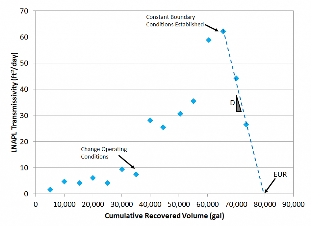
For this evaluation to be valid, the decline rate must be constant. Frequently, the decline rate will change over time due to several factors. When hydraulic recovery is initiated, it takes some time for constant boundary conditions to be established around the well. Typically, the LNAPL recovery rate will increase for a period of time as the LNAPL redistributes around the well, and then the rate will start to decrease. Changes in environmental conditions, such as a fluctuating water table, may affect the decline rate over time. Likewise, changes in operational changes, such as extended downtime periods, may also affect the projections. In these cases, it must be verified that the current conditions are representative of the reasonably anticipated future conditions, and the line should be fit only to the late time data with a constant slope as shown in Figure 2.

Remaining Recoverable Volume
The remaining recoverable volume is the volume of mobile LNAPL that is predicted to be remaining within the radius of influence of the well that can be recovered hydraulically. It is estimated as the difference between the current recovered volume and the EUR.

The remaining time to achieve the EUR can be estimated by incorporating data from a rate-transient decline curve. This evaluation will be presented in an upcoming issue of ANSR.

A Word of Caution
Decline curves require accurate estimation of the volumes and rates of LNAPL recovery. Particular attention must be paid to the estimation of LNAPL volume as it decreases to the limit of measurement. Inconsistent assessment of the volumes associated with an LNAPL sheen, foam, meniscus, or emulsion in the field or the office can have a significant effect on the estimated volume of LNAPL recovered. In some cases, LNAPL transmissivity may be able to provide an accurate decline curve, when recovery rates cannot, by normalizing changes in conditions over time. A thorough understanding of the site conceptual model is also required to ensure the decline observed is due to successful reductions in saturations in the subsurface rather than changes in field condition (such as water table elevation) and/or operational inefficiencies and that the conditions during the period of constant decline are representative of reasonably anticipated future conditions.

References:
Poston, Stephen W. and Bobby D. Poe
2008 Analysis of Production Decline Curves. Society of Petroleum Engineers, 2008.

Sale, Tom
2001 Methods for Determining Inputs to Environmental Petroleum Hydrocarbon Mobility and Recovery Models. American Petroleum Institute Publication Number 4711, July 2001.

Research Corner

Thank you to Dr. Tom Sale of the Colorado State University, Center for Contaminant Hydrology, for providing access to selected graduate level NAPL research.

Resolving Natural Losses of LNAPL Using CO₂ Traps

Kevin M. McCoy
Master of Science
Colorado State University

Abstract: Pools of light non-aqueous phase liquids (LNAPLs) are a legacy of past practices at petroleum facilities. Traditional LNAPL remedies (e.g. hydraulic LNAPL recovery) are often costly and have limited effectiveness. Recent studies have indicated that natural losses of LNAPL can help to stabilize and even shrink subsurface LNAPL bodies once the LNAPL source is removed. Developing an effective understanding of natural losses of LNAPL is an important step in establishing LNAPL management strategies. Estimated rates of natural losses of LNAPL can be used to demonstrate LNAPL stability, form a basis for initiating or discontinuing hydraulic recovery, estimate longevity of LNAPL bodies, and as a benchmark to compare relative effectiveness of different remedial alternatives. Additionally, an understanding of underlying processes gained through field studies can guide development of new, more sustainable LNAPL remediation technologies.

A novel integral CO₂ Trap was created to measure soil CO₂ efflux at grade. This addresses a need for an efficient tool to quantify natural losses of LNAPL. The hypothesis of this thesis is that CO₂Traps can be used to quantify natural losses of LNAPL at field sites. Laboratory and field tests were performed to test the CO₂ Traps and demonstrate their utility.

First, laboratory experiments were undertaken to demonstrate the ability of the traps to quantitatively capture CO₂ and effectively estimate CO₂ fluxes. Closed system column testing showed that the selected sorbent media is capable of quantitatively recovering CO₂. This testing also verified that the sorption capacity of the media (~30% CO₂ by mass) was in the range indicated by the manufacturer. This information is useful when planning maximum field deployment times, and as a means of quality checking field sampling results. Next, an open system column test showed that the CO₂ Traps are capable of quantitatively measuring CO₂ flux through porous media. The traps were field tested. Results of a single round of CO₂ Trap deployment at one field site showed that the traps could distinguish zones of elevated CO₂ flux over the LNAPL body, relative to naturally occurring CO₂ flux at background locations. Background subtracted LNAPL loss rates ranging from 800 to 12,000 gallons per acre per year (gal/acre/yr) were observed. Carbon isotope analysis was performed on one travel blank sample, two background samples, and one LNAPL area sample. Radiocarbon (14C) results provided an independent means to estimate naturally occurring CO₂ flux. Results of the 14C correction agreed well with the background subtraction method for that location.

CO₂ traps have been deployed at a total of 117 locations at 6 field sties. Seasonal resampling of selected locations has yielded a total of 194 CO₂ flux readings. Calculated background corrected LNAPL loss rates for ranged from 400 – 18,000 gal/acre/yr with a mean of 3,500 gal/acre/yr. A detailed analysis of the influence of site and LNAPL characteristics on calculated LNAPL loss rates was performed for one of the six sites. Results indicated that natural losses of LNAPL are largely independent of in-well LNAPL thickness, depth to smear zone, smear zone thickness, or LNAPL type. However, temperature related seasonal trends were observed. Furthermore, natural losses of LNAPL appear to result in self heating of LNAPL zones with a potential benefit of enhancing natural losses. Additional data analysis suggests a link between temperature and natural LNAPL loss rate that may be useful in developing new, more sustainable, LNAPL management technologies.

The primary objective of ANSR is the dissemination of technical information on the science behind the characterization and remediation of Light and Dense Non-Aqueous Phase Liquids (NAPLs).  Expanding on this goal, the Research Corner has been established to provide research information on advances in NAPL science from academia and similar research institutions.  Each issue will provide a brief synopsis of a research topic and link to the thesis/dissertation/report, wherever available.

Practical Stats

Top Twelve Tip #9:
“All models are wrong; some models are useful”
(quoted from G.E.P. Box),
so choose the least hopelessly wrong model

There have been many ways over the years to find the ‘best’ regression model, but today many people still just maximize r-squared.  There are better indicators of a good regression model than that.  Modern indicators are ‘cost benefit analyses’, trading off the gain in decreased model error with the cost of adding new explanatory variables.  r-squared has no cost term built in, so adding an additional x variable always increases r-squared, even if that variable is useless.

Modern indicators of regression quality include Mallow’s Cp, AIC, AICc (AIC corrected) and BIC.  Each is a measure of model error, so that for a given data set the model with the lowest value is the ‘best’.  These indicators can be compared between models with varying numbers and types of explanatory variables, so can be used (for example) to compare a Y= x1 + x3 + x4 model against a Y= x2 + x3 + x5 model, as well as between “nested” models such as Y = x1 + x3 + x4 versus Y = x1 + x2 + x3 + x4.

With modern indicators, modern stat software goes beyond the previous capabilities of stepwise procedures and usually evaluates all the possible regression models with the variables at hand.  Most commercial software as well as the free R system includes “all possible regression” routines.  For example, with 6 explanatory variables there are (2^6-1) = 63 possible regression models:  6 possible one individual x-variable regressions, 15 possible two x-variable regressions, on down to the 1 possible six-variable model.  One or more modern indicators is computed for all 63 models, and the scientist can select from among the best (lowest error) models.  Models near ‘best’ but not the minimum error model may have the advantage based on other considerations, such as cost.  The scientist lets the computer do what it does best, crunch numbers, and the human what it does best, evaluate and make decisions.

“All models are wrong…” tells you to be humble.  Your regression result is only as good as the sampling design and data you have collected.  Even with your best work, you are only estimating relationships in the real world.  You can do better than r-squared.  You can’t be perfect.