Applied NAPL Science Review (ANSR)
Demystifying NAPL Science for the Remediation Manager
Review Board:
J. Michael Hawthorne, PG, Board of Chairman, GEI Consultants, Inc
Mark Adamski, PG, BP America
Andrew Kirkman, PE, AECOM
Diagnostic Gauge Plots
Simple Yet Powerful LCSM Tools
GEI Consultants, Inc.
How do you know if the apparent LNAPL thickness gauged in a well is exaggerated? The answer can mean a substantial difference in predicted LNAPL volumes and associated cleanup costs.
BACKGROUND: As discussed in the last issue (“LNAPL Thickness Revitalized”), LNAPL thickness is an important LNAPL Conceptual Site Model (LCSM) variable. However, the thickness used in multiphase LNAPL volume calculations must be the formation LNAPL thickness (saturation curve height). Under unconfined conditions, apparent LNAPL thickness gauged in wells is a good approximation of the formation LNAPL thickness (mobile LNAPL interval excluding the smear zone). However, confined or perched LNAPL typically results in a substantial exaggeration of apparent LNAPL thickness.
DEFINITION: Diagnostic Gauge Plots are one tool that can be used to determine if LNAPL is unconfined, confined or perched, and to estimate the formation LNAPL thickness. A Diagnostic Gauge Plot is a graph of the air/oil interface (AOI), oil/water interface (OWI) and corrected ground water surface (CGWS) elevations versus the thickness of LNAPL observed in a well over time.
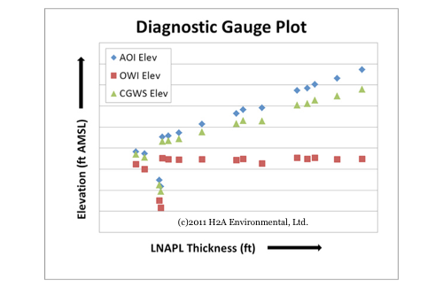
TREND ANALYSIS: Fluctuating AOI, OWI and CGWS elevations in equilibrium will exhibit diagnostic trends when plotted against the associated apparent LNAPL thicknesses gauged in the well. These trends can be used to screen for periods of unconfined, confined or perched LNAPL conditions.
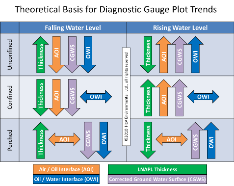
Unconfined LNAPL: During unconfined LNAPL conditions, all three interfaces and the LNAPL thickness will typically fluctuate. The apparent LNAPL thickness will fluctuate in the opposite direction of the three interfaces.
Confined LNAPL: During confined LNAPL conditions, the OWI elevation will typically be stable, and the other three measurements (AOI, CGWS and thickness) will fluctuate, all in the same direction.
Perched LNAPL: During perched LNAPL conditions, the AOI elevation is theoretically stable and the other three measurements (OWI, CGWS and thickness) fluctuate. The apparent LNAPL thickness trend will be opposite to the OWI and CGWS trends.
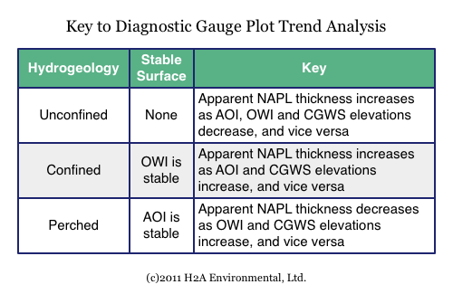
SUMMARY: Under unconfined conditions all three interfaces as well as apparent LNAPL thickness will fluctuate. Under both confined and perched conditions, one interface will be stable, but the other two interfaces and the apparent thickness will fluctuate. The key is to identify which interface is stable, and whether apparent thickness and the fluctuating interface elevations are moving together or in opposite directions.
ADVANCED: If multiple hydrostatic conditions exist over time for a given well, then multiple trends will be observed in that well’s Diagnostic Gauge Plot. In such cases, the points of inflection where trends change direction can be used to estimate LNAPL formation thickness.
REAL WORLD LIMITATIONS: A word of caution – non-equilibrium conditions, vertical gradients, and other factors can affect the results of a Diagnostic Gauge Plot analysis. For example, routine product removal events through bailing or other means can prevent the attainment of equilibrium conditions in wells with LNAPL. As a result, the non-equilibrium gauging data may not follow the ideal theoretical trends for Diagnostic Gauge Plots. Multiple lines of evidence should be used.
Next month’s issue will explore Hydrostratigraphs, another diagnostic LNAPL Conceptual Site Model tool that can be used to confirm the results of a Diagnostic Gauge Plot analysis.
Until then, feel free to call or email with questions regarding the use of Diagnostic Gauge Plots in modern day LNAPL science to minimize your site remediation costs.