Calculating NAPL Drawdown
Volume 4, Issue 3 | September 2014

Download PDF

Applied NAPL Science Review

Demystifying NAPL Science for the Remediation Manager

Editor: J. Michael Hawthorne, PG

Asst. Editor: Dr. Rangaramanujam Muthu

ANSR Scientific Advisory Board
J. Michael Hawthorne, PG, Board of Chairman, GEI Consultants Inc.
Mark Adamski, PG, BP Americas
Stephen S. Boynton, PE, LSP, Subsurface Env. Solutions, LLC
Dr. Randall Charbeneau, University of Texas
Paul Cho, PG, CA Regional Water Quality Control Board-LA
Robert Frank, RG, CH2M Hill
Dr. Sanjay Garg, Shell Global Solutions (US) Inc.
Randy St. Germain, Dakota Technologies, Inc.
Dr. Dennis Helsel, Practical Stats
Dr. Terrence Johnson, USEPA
Andrew J. Kirkman, PE, BP Americas
Mark Lyverse, PG, Chevron Energy Technology Company
Mark W. Malander, ExxonMobil Environmental Services

Applied NAPL Science Review (ANSR) is a scientific ejournal that provides insight into the science behind the characterization and remediation of Non-Aqueous Phase Liquids (NAPLs) using plain English. We welcome feedback, suggestions for future topics, questions, and recommended links to NAPL resources. All submittals should be sent to the editor.

Calculating NAPL Drawdown

Light non-aqueous phase liquid (LNAPL) transmissivity is a powerful metric to quantify and assess the recoverability of mobile non-aqueous phase liquid (NAPL). Numerous techniques for the estimation of LNAPL transmissivity exist (ASTM 2013). Many require an accurate calculation of NAPL drawdown to calculate accurate NAPL transmissivity values. NAPL drawdown can be induced by gravity pumping and/or by the addition of vacuum. This article focuses solely on gravity pumping drawdown; vacuum induced drawdown will be addressed in a future article.

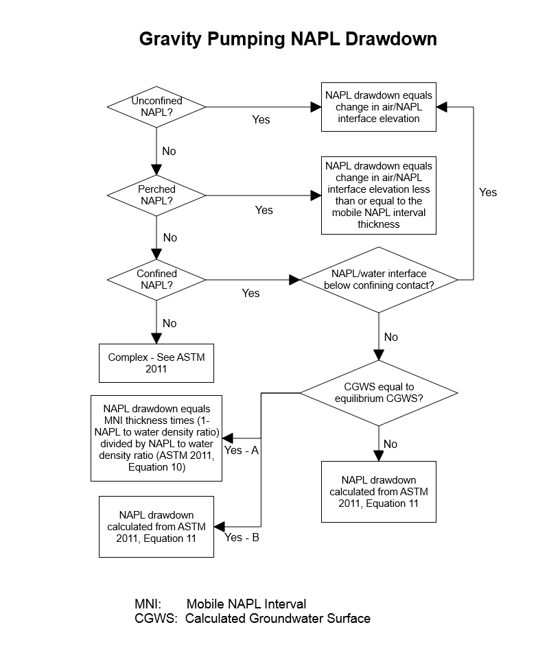
NAPL drawdown is calculated differently depending upon whether the NAPL is unconfined, perched, or confined (ASTM 2013). For unconfined NAPL, drawdown is simply the change in the air/NAPL (AN) interface induced by the removal of fluids from a well (such as, during a baildown test). For perched NAPL, drawdown is also the change in the AN interface induced by fluids removal, but the maximum drawdown used to calculate NAPL transmissivity cannot exceed the formation mobile NAPL interval thickness (unless vacuum is applied). For confined NAPL, the depth of the NAPL/water (NW) interface in relation to the confining contact will dictate the calculation method (up to three different equations) that could be used to estimate drawdown (Figure 1).

Figure 1 – Flow chart for the calculation of NAPL drawdown under differing NAPL hydrogeologic conditions.

Unconfined NAPL

Unconfined NAPL drawdown is calculated as the change between the equilibrium AN interface elevation and the transient AN interface elevations as the NAPL recharges into the well and the AN interface elevation gradually rises back to its initial equilibrium elevation (Figure 2).

Figure 2 – Depiction of equilibrium and drawdown conditions for unconfined NAPL.

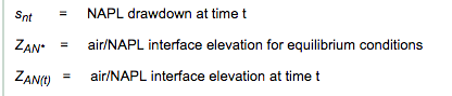
The equation for calculation of NAPL drawdown under unconfined conditions is fairly simple:

ASTM 2013, Equation 9:

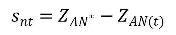
Where:

Perched NAPL
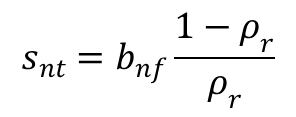
Perched NAPL drawdown is calculated identically to unconfined NAPL drawdown so long as the drawdown does not exceed the formation mobile NAPL interval thickness. However, it is possible for the apparent NAPL drawdown to exceed the perched mobile NAPL interval thickness. In this case, the maximum NAPL drawdown is calculated as the difference between the equilibrium air/NAPL (AN) interface elevation and the elevation of the perching layer (ASTM 2013) (Figure 3).

Figure 3 – Depiction of equilibrium and drawdown conditions for perched NAPL.

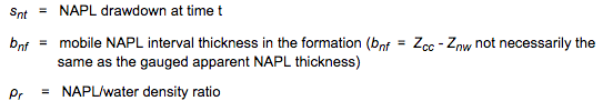
The equation for calculation of NAPL drawdown under perched NAPL conditions is:

ASTM 2013, Equation 9:

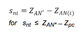
Where:

Confined NAPL

Estimating confined NAPL drawdown can be considerably more complex than either unconfined or perched drawdown. The three possible conditions (all of which could potentially exist in a single NAPL transmissivity test) vary with the elevations of the NAPL/water (NW) interface relative to the confining layer and the location of the calculated groundwater surface (CGWS) during recharge relative to the equilibrium CGWS (Figure 4). The three conditions include:

1. NAPL/water (NW) interface below confining contact regardless of air/NAPL (AN) interface or CGWS location;
2. NAPL/water (NW) interface above confining contact and CGWS at equilibrium; and
3. NAPL/water (NW) interface above confining contact and CGWS below equilibrium.

Figure 4 – Depiction of equilibrium and three possible confined drawdown conditions for confined NAPL.

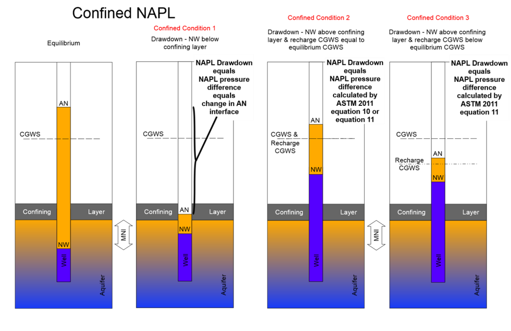
Confined condition 1 – Regardless of where the air/NAPL (AN) interface or the CGWS occur, if the NAPL/water (NW) interface is below the confining contact, then the NAPL in the well is in contact with the NAPL in the formation, and NAPL drawdown is calculated the same as for unconfined NAPL (ASTM 2013). This remains true even if groundwater extraction creates an unconfined condition and pulls the air/NAPL (AN) interface and CGWS below the confining contact. By definition, at that point, the NAPL is unconfined and drawdown is calculated based on the change in air/NAPL (AN) interface.

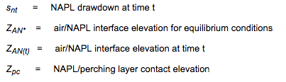
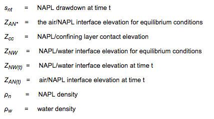
Confined condition 2 – If the NAPL/water (NW) interface is above the confining contact and the CGWS is at equilibrium, then NAPL in the well is not in contact with the formation mobile NAPL interval, the fluid distribution pressure across the mobile NAPL interval remains constant, and NAPL discharge into the well is constant and is balanced by an equivalent mass of water discharge out of the well (ASTM 2013). In this case, either the simplified drawdown equation (ASTM 2013, Equation 10) or the generalized confined drawdown equation (ASTM 2013, Equation 11) may be used.

ASTM 2013 Equation 10 (simplified confined drawdown equation):

Where:

ASTM 2013 Equation 11 (generalized confined drawdown equation):

Where:

Confined condition 3 – If the NAPL/water (NW) interface is above the confining contact and the CGWS is below the equilibrium CGWS, then NAPL in the well is not in contact with the formation mobile NAPL interval and the fluid distribution pressure across the mobile NAPL interval is not constant. In this case, the simplified drawdown equation (ASTM 2013, Equation 10) may NOT be used, but the generalized confined drawdown equation (ASTM 2013, Equation 11, above) is still valid. This equation is accurate regardless of whether the CGWS is at or below equilibrium because it calculates the pressure difference at the top of the mobile NAPL interval and then converts it into NAPL head or NAPL drawdown.

Remember that ultimately NAPL drawdown is an analogue for the pressure difference between the mobile NAPL interval in the formation and the apparent NAPL thickness and corresponding interface elevations in a well. A detailed LCSM is crucial to correctly understanding NAPL hydrogeologic conditions and the mobile NAPL interval in the formation, and then correctly calculating NAPL drawdown. For assistance in recognizing and working with NAPL under various hydrogeologic conditions, refer to (Kirkman et al. 2013), (Hawthorne 2011), (Hawthorne and Kirkman 2011), (Hawthorne et al. 2011a), (Hawthorne et al. 2011b), (Adamski 2012), and (Hawthorne 2014).

A Word of Caution: NAPL drawdown is a critical parameter for the calculation of LNAPL transmissivity. The induction of a large vacuum or excessive water-induced drawdown to a well does not consistently get transmitted through the well screen and filter pack to the NAPL. This can be due to many factors such as heterogeneity, head loss through the filter pack (vacuums especially), and fluid interference or smearing. Pilot testing can provide a good indication of the limits where increased drawdown does not induce increased fluid flow. Errors in the calculation of NAPL drawdown will result in errors in the calculation of NAPL transmissivity. If a clear understanding of NAPL hydrogeologic conditions and the mobile NAPL interval is unknown then it is unlikely that accurate drawdown or transmissivity calculations will be achieved.

References:
Adamski, Mark
2012 Mechanisms for LNAPL to Enter Confined Conditions (Volume2, Issue 4), June 2012.

ASTM
2013 Standard Guide for Estimation of LNAPL Transmissivity. ASTM E2856-13. ASTM International, West Conshohocken, PA.

Hawthorne, J. Michael
2011 Diagnostic Gauge Plots (Volume 1, Issue 2), February 2011.

Hawthorne, J. Michael
2014 Site Wide Analysis of LNAPL Distribution and Hydrogeologic Conditions Using Plume Scale Diagnostic Gauge Plots (Volume 4, Issue1), January 2014.

Hawthorne, J. Michael, and Andrew J. Kirkman
2011 Discharge vs. Drawdown Graphs (Volume 1, Issue 4), April 2011.

Hawthorne, J. Michael, Mark Adamski, Sanjay Garg, and Andrew J. Kirkman
2011a Confined LNAPL (Volume 1, Issue 5), May 2011.

Hawthorne, J. Michael, Mark Adamski, Sanjay Garg, and Andrew J. Kirkman
2011b Perched LNAPL(Volume 1, Issue 6), June 2011.

Kirkman, Andrew J., Mark Adamski, and J. Michael Hawthorne
2013 Identification and Assessment of Confined and Perched LNAPL Conditions, Groundwater Monitoring & Remediation, Volume 33, Issue 1, pp 75-86.

Research Corner

Thank you to Dr. Tom Sale of the Colorado State University, Center for Contaminant Hydrology, for providing access to selected graduate level NAPL research.

Thermal aspects of STELA (sustainable thermally enhanced LNAPL attenuation)

Click to download thesis

Daria Akhbari

Master of Science

Colorado State University

Abstract: Extensive bodies of light non-aqueous phase liquids (LNAPLs) are commonly found beneath petroleum facilities.  Related concerns include lateral spreading of LNAPL, impacts to groundwater, and impacts to indoor air.  Recent studies have shown that natural losses of LNAPL can be on the order of thousands of gallons per acre per year and temperature is a primary factor controlling rates of natural losses.  Results of the laboratory and field experiments suggest that LNAPL impacted media in the range of 18-300C can have loss rates that are an order of magnitude greater than media at temperatures less than 18ºC.  The vision that has emerged from recent work is that passive thermal management strategies could enhance natural losses of LNAPL and significantly reduce the longevity of LNAPL.  Owing to this new understanding, plans were developed for a small-scale field demonstration of sustainable thermally enhanced LNAPL attenuation (STELA) at a former refinery in Wyoming, located adjacent to the North Platte River.  The overarching objective of the STELA initiative is to develop a new technology for LNAPLs that is more effective, faster, more sustainable, and/or lower cost than current options.  The primary objective of the field demonstration is to collect data needed to evaluate cost and performance at field sites.  In November 2011, seventeen multilevel sampling systems were installed in a 10m by 10m area.  Preheating temperature and water quality data were collected through the multilevel samplers over a period of 10 months.  In August 2012, ten heating elements, including submersible heat trace wires wrapped around 7.6 cm ID PVC pipe with thermostat controls, were installed upgradient of the sampling network to deliver heat to sustain subsurface temperature in an LNAPL body.  The heating elements were energized in September 2012.  Subsequently, effects of the heating elements on the subsurface temperature were monitored using 17 multilevel sampling systems equipped with 6 thermocouples for 10 months. Preheating data indicates that in the absence of heating, subsurface temperatures are in the range of 18-30°C for 40 days per year.  Data collected from September 2012 to July 2013 indicates that with heating, conditions can be maintained in the target range for 60 to 200 days per year depending upon proximity to the heat source.  A principle challenge is heat loss to the surface in the winter.  Minimum and maximum power inputs have been 15 kw-hr/day and 30 kw-hr/day occurring, respectively in October and May.  Assuming an energy cost of 0.10 kw-hr, this equates to costs of 1.5 $/day to 3 $/day.  An independent experiment using Geo-net layer showed that using Gas Permeable Insulation/Heat Sink (GPIHS) system has the potential to enhance the ability of the heating system to sustain temperature beneath the ground surface, and, potentially decrease the power costs.  A primary challenge with evaluation and design of STELA systems is anticipating the appropriate spacing of heating elements and necessary energy inputs.  Herein this challenge is met by developing a model, calibrated to field data, which can be used to design a full-scale STELA remedies.  The overarching objective of the modeling is to demonstrate methods that can be employ to evaluate and/or design full-scale STELA systems.  At 5m downgradient of the heating elements, the developed model, accurately, predicted 60 days of the effective season in 2012.  Also, the simulation results anticipate that by keeping the heating system activated for three years, the effective season will increase each year.  At 5m downgradient of the heating elements, model results suggested 120 days and 150 days of effective season for 2013 and 2014, respectively as compared to 60 days in the first year.  The ability of the model to anticipate the effective season for the next years makes the model a useful tool to design and evaluate the future STELA systems.  Calibration of the model to the field data shows that exothermic reactions associated with LNAPL losses can change the heat distribution at the system.  In addition, the simulation results indicate that the losses at the subsurface are in the range of 5,000 to 10,000gal/acre/yr.  These anticipated loss rates are consistent with the previous values reported by McCoy (2012) in 2012 (~900-11,000gal/acre/yr).  A conceptual STELA design is developed in the last chapter to explore the cost of a STELA system at a 1-hectare site.  The design is based on condition at the former refinery in Wyoming where the STELA field demonstration was conducted.  The cost analysis study indicated that the primary cost is the heating elements installation.  The second significant cost is the operation costs, and the third significant cost that can be reduced is the energy source.  The cost estimates normalized to common units indicated that the total cost ranges between $590,000 to $720,000 per hectare, $11.9 to $14.4 per cubic meter of treated soil, and $1.3 to $1.5 liter of LNAPL removed depends on the energy source, heating system and the degradation rate.  Cost of this magnitude support the hypothesis that STELA has the potential to have cost that is lower than other options employed for LNAPL remediation.

The primary objective of ANSR is the dissemination of technical information on the science behind the characterization and remediation of Light and Dense Non-Aqueous Phase Liquids (NAPLs).  Expanding on this goal, the Research Corner has been established to provide research information on advances in NAPL science from academia and similar research institutions.  Each issue will provide a brief synopsis of a research topic and link to the thesis/dissertation/report, wherever available.

Practical Stats

Top Twelve Tip #2:

Treat Outliers Like Children: correct them when needed, but never throw them out

Dr. Dennis Helsel
www.practicalstats.com

Many scientists perform outlier tests such as Grubbs or Rosner tests to determine whether an observation is an outlier.  Then they toss the observation away if it is.  Outlier tests determine only whether an observation is likely to have been generated from a normal distribution.  Most field data in environmental sciences are skewed, and do not look like a normal distribution.  The simple fact that most data collected in the field have a zero lower bound introduces skewness, just as in the data here.  There is no reason to suspect that they should look like a normal distribution.  Rejecting that the top one or few observations come from a normal distribution is no reason to label those observations ‘bad’ and toss them away.  They probably cost a great deal of time and money to collect, and are the product of that scientist’s good work.

A box plot of 23 observations shows one ‘outlier’ by the Dixon test.

If logarithms or cube roots of the data were taken, the top observation would not test as a significant outlier.  Can an observation be ‘bad’ in one measurement scale but ‘good’ in another?  The top observations often rate as not coming from a normal distribution.  For environmental science, that’s ‘normal’. Don’t be quick to toss your data away, and most importantly, base that decision on science (where and when the data were collected, perhaps) rather than on a statistical test.  There is no test for ‘badness’ in statistics.