Calculating Mole Fractions from LNAPL and Soil Samples
Volume 5, Issue 1 | March 2015

Download PDF

Applied NAPL Science Review

Calculating Mole Fractions from LNAPL and Soil Samples

Editor: J. Michael Hawthorne, PG

Asst. Editor: Dr. Rangaramanujam Muthu

ANSR Scientific Advisory Board
J. Michael Hawthorne, PG, Board of Chairman, GEI Consultants Inc.
Mark Adamski, PG, BP Americas
Stephen S. Boynton, PE, LSP, Subsurface Env. Solutions, LLC
Dr. Randall Charbeneau, University of Texas
Paul Cho, PG, CA Regional Water Quality Control Board-LA
Robert Frank, RG, CH2M Hill
Dr. Sanjay Garg, Shell Global Solutions (US) Inc.
Randy St. Germain, Dakota Technologies, Inc.
Dr. Dennis Helsel, Practical Stats
Dr. Terrence Johnson, USEPA
Andrew J. Kirkman, PE, BP Americas
Mark Lyverse, PG, Chevron Energy Technology Company
Mark W. Malander, ExxonMobil Environmental Services

Applied NAPL Science Review (ANSR) is a scientific ejournal that provides insight into the science behind the characterization and remediation of Non-Aqueous Phase Liquids (NAPLs) using plain English. We welcome feedback, suggestions for future topics, questions, and recommended links to NAPL resources. All submittals should be sent to the editor.

Calculating Mole Fractions
from LNAPL and Soil Samples

One of the primary components of an LNAPL site conceptual model is characterization of LNAPL chemistry (ASTM 2006), often including the mole fractions of individual constituents. Mole fractions are important because they help in predicting constituent (e.g., benzene) concentrations in groundwater and soil gas that contact the LNAPL. Also, decreasing mole fractions over time are an indication of source zone depletion.

LNAPL Samples
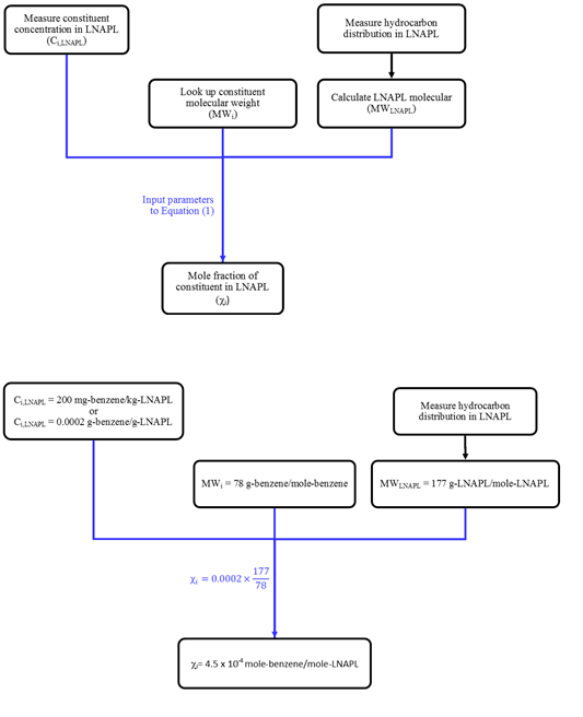
A typical mole fraction calculation is based on analytical results for an LNAPL sample.

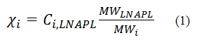
Where:

The C_i,LNAPL term is reported by the laboratory from a gas chromatograph / mass spectrometry analysis (e.g., GC/MS by EPA 8260B), and the practitioner simply needs to convert from the units reported by the laboratory (typically mg/kg) to those in the above equation (g/g). The MW_i term is a known value based on the molecular formula of the constituent.

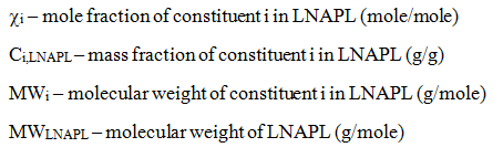
This leaves the MW_LNAPL term. Molecular weights for LNAPLs can vary by a factor of 2 or 3, so it is worth obtaining an estimate of this value for a given sample. One estimation method is based on the carbon distribution of the LNAPL, obtained from a simulated distillation analysis (e.g., ASTM D3710). In a simulated distillation, the LNAPL is boiled at sequentially higher temperatures that are referenced to known chemical standards, typically aliphatic hydrocarbons (Villalanti et al. 2000). An example laboratory that performs simulated distillation and reports carbon numbers as mass fractions is Energy Laboratories (Billings, MT).

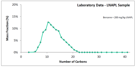
In the above simulated distillation plot, the mass fraction of the LNAPL has been quantified for all C_n from C₃ to C₄₂. The molecular weight of this LNAPL can be estimated, so long as an assumed hydrocarbon structure corresponding to each carbon number is made. An all-aliphatics assumption is expected to have a maximum error of approximately 10% (e.g., an overestimate for LNAPLs that are actually comprised of all aromatics). Figure 2 assumes an aliphatic hydrocarbon structure with molecular formula C_nH_2n+2. For instance, C₁₀ is assigned a hydrocarbon weight of 142 g/mole corresponding to C₁₀H₂₂. Each hydrocarbon weight is then multiplied by the mass fraction, such as 142 g/mole x 9% mass fraction = 13 g/mole for C₁₀. The multiplied values are listed as data labels on Figure 2. The values summed give the LNAPL molecular weight.

For the laboratory-reported benzene content of 200 mg/kg in the LNAPL sample, and calculated 177 g/mole molecular weight, the corresponding benzene mole fraction is 4.5 x 10^-4 mole/mole. The calculation steps are shown on Figure 3.

Soil Samples
There are times when LNAPL samples cannot be obtained from wells. For instance, at some sites LNAPL may not enter existing wells because LNAPL saturations within the formation are at or below residual values, or wells are not screened across the zone of mobile LNAPL. At other sites, wells may not be located in areas with LNAPL. It is still possible to estimate the mole fractions of individual constituents in the smear zone LNAPL, but in these cases smear zone soil samples can be collected instead of LNAPL samples.

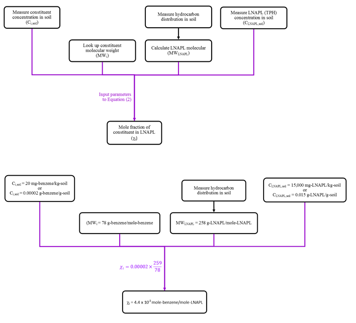
The procedure to estimate mole fractions for soil samples is similar to that for LNAPL samples, with one extra conversion step. This calculation requires the fundamental assumption that the

hydrocarbons in sampled soil are present as LNAPL. The practitioner should check that LNAPL is present during sample collection, measured total petroleum hydrocarbon (TPH) concentrations are sufficiently high, and/or that individual constituents are above soil saturation values (EPA 1996). The mole fraction of constituent i can then be estimated by:

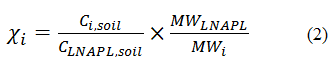
Where:

The C_i,soil term can be measured by the laboratory using the same GC/MS methods for soil as for LNAPL. The C_LNAPL,soil term can be measured by a TPH analysis (e.g., GC/flame ionization detector EPA 8015B or by GC/MS; Haddad and MacMurphey 1997). Note that, if a GC/FID method is used, then the C_i,soil and C_LNAPL,soil laboratory analyses will necessarily be conducted on different soil aliquots. This introduces some uncertainty to the mole fraction estimates due to possible soil heterogeneity.

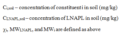
Close communication with the laboratory is required when obtaining carbon distributions via soil samples to estimate the MWLNAPL term. The laboratory must report not just a TPH value for soil, but also the carbon distribution for that TPH value. Terms used by laboratories include “custom TPH ranges” (Lancaster Laboratories, Lancaster, PA), “TPH carbon chains,” and “carbon series” (BC Laboratories, Bakersfield, CA). Whatever the terminology by the laboratory, they must understand that the mass fractions of carbon numbers within a TPH value are to be reported. The amount of carbon number discretization varies from laboratory to laboratory. An example for a laboratory that provides only moderate discretization is shown on Figure 4.

The laboratory in the above example reported only six carbon groups: C₆-C₉, C₁₀-C₁₂, C₁₃-C₁₆, C₁₇-C₂₂, C₂₃-C₂₈, and C₂₉-C₄₀. While the degree of discretization is smaller than that for a simulated distillation, it still allows for an LNAPL molecular weight estimate that is likely superior to simply referencing one based on expected product types. A nominal aliphatic carbon number can be assumed for each of the reported ranges (e.g., C₁₁ for C₁₀-C₁₂) and the LNAPL molecular weight estimated. The maximum expected error for the below example is approximately 20% (e.g., for carbon numbers different than those assumed).

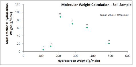
For the above example, an estimated molecular weight is 259 g/mole. For the laboratory-reported 20 mg/kg benzene and 15,000 mg/kg TPH concentrations in soil, the corresponding benzene mole fraction in LNAPL would be 4.4 x 10^-3 mole/mole. The calculation steps are shown on Figure 6.

A Word of Caution: The estimated mole fractions for soil samples likely have more uncertainty than those for LNAPL samples due to possible effects from soil heterogeneity and lower degrees of carbon number discretization. However, soil samples can be collected from multiple depths in a smear zone, providing an advantage to LNAPL samples collected from wells. Regardless of the method used, it is important to do a check with other methods, such as by calculating effective solubilities based on mole fractions and then comparing to measured groundwater concentrations. A robust LNAPL site conceptual model uses parameter values derived from multiple methods.

References:
ASTM
2006 Standard Guide for Development of Conceptual Site Models and Remediation Strategies for Light Nonaqueous-phase Liquids Released to the Subsurface. ASTM E2531-06e1. ASTM International, West Coshohocken, PA.

EPA
1996 Soil Screening Guidance: Technical Background Document. EPA/540/R95/128. Office of Solid Waste and Emergency Response, Washington, D.C.

Haddad, Robert. and John MacMurphey
1997 TPH measurements: The advantage of using GC/MS. Proceedings of the 1997 Petroleum Hydrocarbons and Organic Chemicals in Groundwater: Prevention, Detection, and Remediation Conference, 197–206.

Villalanti, Dan C., Joseph C. Raia, and Jim B. Maynard.
2000 High-temperature simulated distillation applications in petroleum characterization. In Encyclopedia of Analytical Chemistry R.A. Meyers (Ed.). John Wiley & Sons Ltd, Chichester. pp. 6726-6741.

Research Corner

Thank you to Dr. Tom Sale of the Colorado State University, Center for Contaminant Hydrology, for providing access to selected graduate level NAPL research.

Evaluation of Three Methods for Estimating Formation Transmissivity to LNAPL

Gabriel Charles Iltis
Master of Science
Colorado State University

Abstract: Light non-aqueous phase liquids (LNAPLs) are persistent sources of groundwater contamination commonly encountered beneath petroleum refining, transmission, and storage facilities. The primary concerns associated with LNAPL contamination include the potential for LNAPL migration as a separate liquid phase and groundwater contamination resulting from dissolution of LNAPL constituents into the aqueous phase. The potential for LNAPL migration is dependant on the soil formation transmissivity to LNAPL. This thesis compares the relative merits of three methods of estimating formation transmissivity to LNAPL, including baildown tests, petrophysical methods, and single-well tracer dilution techniques.

Over the last twenty years, a number of techniques have been developed to characterize formation transmissivity to LNAPL. Two of the most commonly utilized methods are baildown tests and petrophysical methods. In addition, Colorado State University (CSU) has developed a down-well probe that enables the implementation of single-well tracer dilution techniques within LNAPL present in a well screen. This technology provides a discrete measurement of the in-situ flow rate of LNAPL through the well screen. Given the local LNAPL gradient, measured in situ flow rates can be transformed to formation LNAPL transmissivity values. The results of laboratory testing conducted in a two-dimensional sand tank suggest that estimates of LNAPL transmissivity obtained from both baildown and tracer dilution techniques compare reasonably well to known values based on Darcy’s equation (92.2 and 88.2% of the Darcy’s equation value respectively). Laboratory scale petrophysical analysis tended to underestimate LNAPL transmissivity resulting in values that are
22.2 to 47.7% of the Darcy’s equation values. Petrophysical analysis was conducted using both the Brooks-Corey and van Genuchten capillary pressure-saturation models, and two saturated hydraulic conductivity values. The primary limitation of the laboratory scale petrophysical analysis is the accuracy of the permeability values determined using disturbed soil samples and laboratory permeameters. Test methods for evaluating formation transmissivity to LNAPL were also compared at a single field location (well SS-146) in Evansville, Wyoming. Field baildown tests were evaluated using two methods: the modified Bouwer-Rice method, and the Cooper-Jacob method. Bouwer-Rice analysis of a single data set estimated LNAPL transmissivity to be 3 cm²/min. Two sets of test data, analyzed using the Cooper-Jacob method yielded transmissivity values of 0.3 cm²/min and 1.8 cm²/min. Tracer dilution testing evaluated the LNAPL transmissivity to be 0.06 cm²/min. Petrophysical analysis yielded transmissivity values varying by six orders of magnitude (3.6E-5 to 5.2 cm²/min). The large variation reflects differences in hydraulic conductivity values obtained from an aquifer test (high end) and laboratory permeameter studies (low end). For the field study, there is no reference value for LNAPL transmissivity with which to evaluate accuracy of each method. The primary issue associated with baildown testing is the subjectivity of data analysis and potential changes in fluid saturations local to the well associated with the testing procedure. The limitation of the tracer dilution technique is the dependence of the method on accurate resolution of the LNAPL gradient through the well. The potential for inaccuracies in analysis of field properties using ex situ laboratory tests is the primary limitation of petrophysical analysis. Given the conditions evaluated in this thesis, the baildown test methods provide the most reasonable estimates of formation transmissivity to LNAPL. In comparison, the tracer dilution technique is constrained (in field applications) by the accuracy to which the local LNAPL gradient can be evaluated. However, the tracer dilution techniques do not have this limitation if one is interested in determining, directly, the rate of LNAPL flow. Lastly, petrophysical methods are constrained by the accuracy to which estimates of in situ soil parameters can be determined using disturbed soil specimens and ex situ
laboratory test methods.

The primary objective of ANSR is the dissemination of technical information on the science behind the characterization and remediation of Light and Dense Non-Aqueous Phase Liquids (NAPLs). Expanding on this goal, the Research Corner has been established to provide research information on advances in NAPL science from academia and similar research institutions. Each issue will provide a brief synopsis of a research topic and link to the thesis/dissertation/report, wherever available.

Practical Stats

Top Twelve Tip #4:
Transforming data requires transforming solutions

Dr. Dennis Helsel
www.practicalstats.com

Transformations have been used for 3 purposes in statistics (not just by whim):

1. to make data more like a normal distribution
2. to make data relationships more linear
3. to make data more constant in variance

These are requirements of traditional, parametric tests. Logarithms often better meet these objectives due to the skewness of environmental data. Taking logs has been popular due to their relatively simple mathematics, and their flexibility in fitting a wide range of data shapes. But what does this do to the interpretation of the test result?

Specific capacity, a standardized measure of yields of water from wells, was measured in hundreds of wells across the Appalachian region of the US in a USGS report of the late 1980s. This is a dataset we’ve used for years in our Applied Environmental Statistics course. The data come from four rock types, and there was strong interest in learning if well yields differed between the four rock units. Figure 1 shows boxplots of the original data, while Figure 2 shows boxplots of the logarithms of the same data.

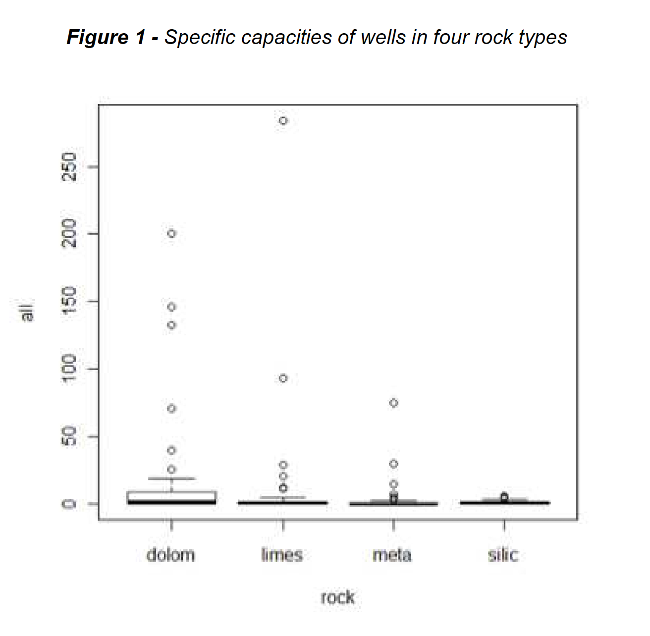
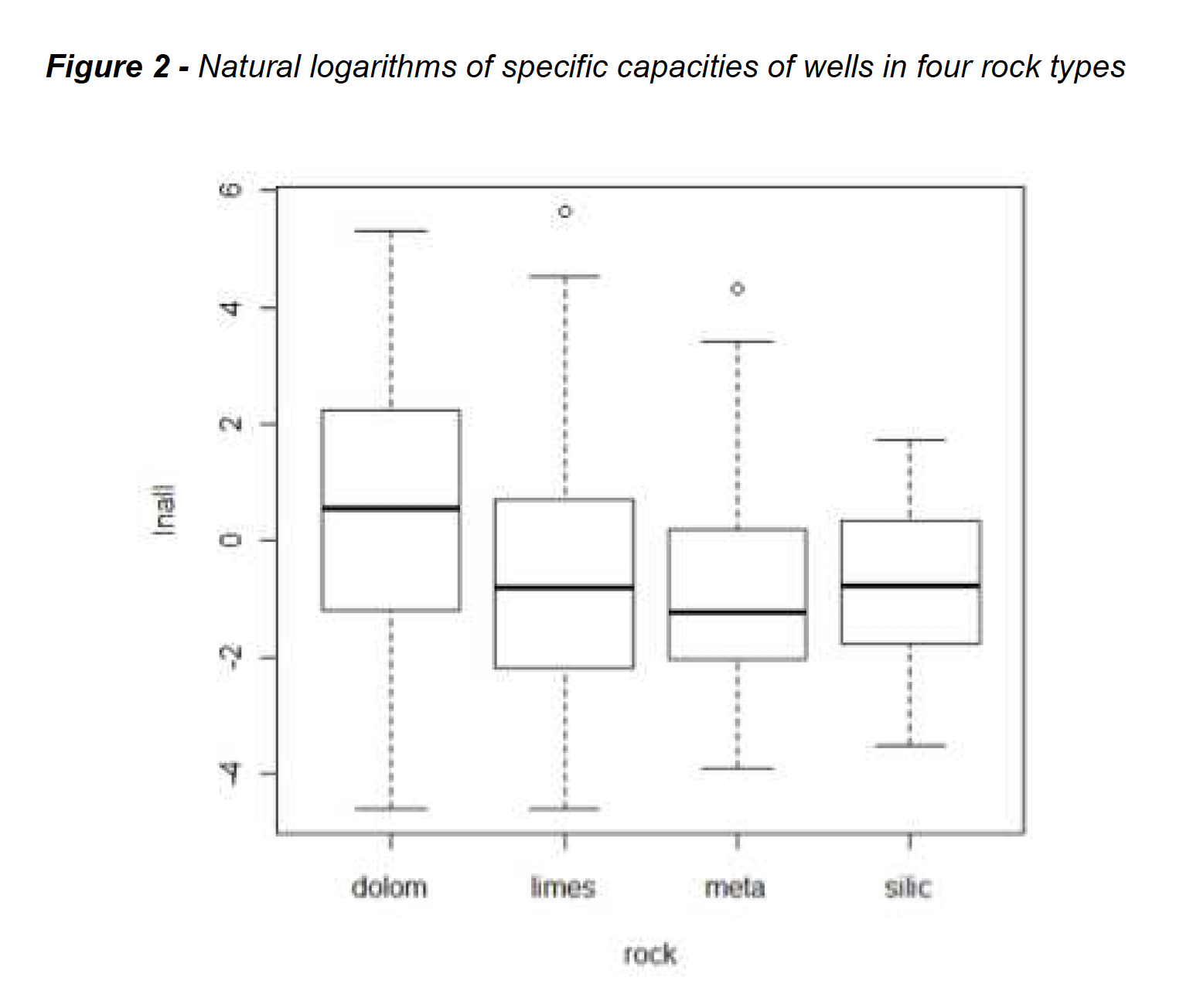
As can be seen, the boxplots of logarithms appear of about the same heights (same variability of data) and similar to a normal distribution – top and bottom portions of the boxes are about the same size, with few outliers. Boxplots of the specific capacities themselves in Figure 1 do not have these characteristics, and these data do not appear to follow normal distributions. Common parametric tests such as analysis of variance (ANOVA) require data to follow a normal distribution and each group have the same variance. Otherwise, the tests have low power – low ability to see differences that are present.

ANOVA tests differences between group means. On the original Figure 1 data the ANOVA p-value is 0.08, so group means would not be considered different. Is the non-normality causing a loss of power, pushing up the p-value, even with 50 observations in each group? ANOVA on the logarithms of Figure 2 gives a p-value of 0.007. However, this test is not a test of differences in the mean specific capacity! It tests whether the mean of the logarithms differs between groups. The mean of the logarithms is called the geometric mean when retransformed back to original units. The geometric mean is one way to estimate the median, not the mean, of the data in original units. By computing the test in log units, we are testing the difference between geometric means — testing the difference in medians of the groups rather than their means. A Kruskal-Wallis (nonparametric) test of group medians has a similar p-value of 0.009, another indication that medians are being tested by the ANOVA on logs.

If you transform data you must transform your idea of what is being tested with a parametric test. Means are ‘unit-specific’, and whether performing hypothesis tests, regression, or confidence intervals, what is being targeted changes once logarithms are used. Often what we actually want is a test of medians (“is one group different than the others?”). But if we specifically want to test means, transformations destroy that. There are newer methods than analysis of variance to test differences in means without assuming a normal distribution. These are called permutation tests. The permutation p-value (using the untransformed data) is 0.04 irrespective of the data’s shape, stating that group means do differ for these data.

The difference in p-value between the permutation (0.04) and classical ANOVA (0.08) tests in original units is the loss of power for classical ANOVA. As here, a better test can see something the older tests cannot. If you’d like to learn more about permutation tests, we offer both webinars and in-person courses on how they work and how they can help your data analysis come into the 21st century. See https://practicalstats.com/training for more information.