J. Michael Hawthorne, PG, Board Chairman, GEI Consultants, Inc.
Andrew J. Kirkman, PE, BP Corporation North America
Robert Frank, RG, Jacobs
Paul Cho, PG, CA Regional Water Quality Control Board-LA
Randy St. Germain, Dakota Technologies, Inc.
Dr. Terrence Johnson, USEPA
Brent Stafford, Shell Oil Co.
Douglas Blue, Ph.D., Imperial Oil Environmental & Property Solutions (Retired)
Natasha Sihota, Ph.D., Chevron
Kyle Waldron, Marathon Petroleum
Danny D. Reible, Professor at Texas Tech University
Reeti Doshi, National Grid
Mahsa, Shayan, Ph.D., PE, AECOM Technical Services
Frequently Asked Questions
DISCLAIMER: This article was prepared by the author(s) in their personal capacity. The opinions expressed in this article are the author’s own and do not necessarily reflect the views of Applied NAPL Science Review (ANSR) or of the ANSR Review Board members.
Large Scale – Homogeneous Soil Example
To make this more engaging let’s play a game where you are shown light NAPL (LNAPL) release characterization data, and then you define the associated LNAPL body shape.
Let’s first discuss the rare case where geologic heterogeneity is NOT influencing the LNAPL release. The reader might want to print this article out on paper and draw the LNAPL body outlines right over the data figures. Avoid peaking ahead at subsequent figures though, because they’ll contain the true LNAPL body “reveals”.
This example follows a typical LNAPL characterization sequence:
- Examine evidence gathered from wells/logging data (assume “ideal” tools and methodologies were used).
- Develop the LNAPL CSM (LCSM).
- Attempt to explain the LCSM if at all possible.
The first release site (Figure 1) includes the following data:
- No scale is shown (actual scale isn’t important for this)
- Groundwater (GW) elevations
- LNAPL point of release (POR)
- Five “nests” of data including:
- monitoring wells (left side of each nest) – dashes indicate the well screen – yellow fill indicates the gauged LNAPL thickness
- soil permeability (center)
- LNAPL logging data (right side) – red fill indicates formation LNAPL (intensity denotes observed abundance)
These data are typical of the “multi-purpose” approach to characterizing LNAPL in that the well installations not only generate the required dissolved phase GW data, but formation LNAPL data as well.
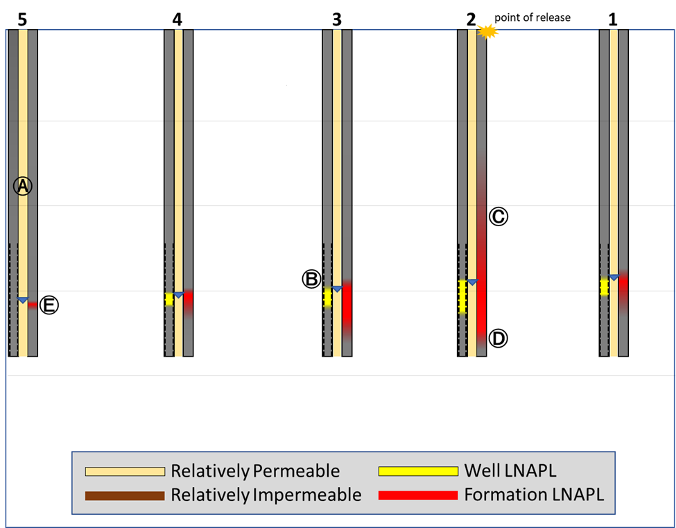
A. Site soil is remarkably homogenous and readily conducts fluids.
B. GW table surface is sloped down toward the left.
C. LNAPL just below the release point is present in the formation, above the GW surface.
D. LNAPL is present in the formation below the GW surface – deepest observations are directly below the release and the penetration tapers with lateral distance from the release point.
E. The monitoring well LNAPL data are consistent with formation LNAPL, only smaller. The single exception is nest #5 where LNAPL is present in the formation but was not observed in the well.
Now draw some dashed “LNAPL extent” lines for: 1. Well LNAPL and 2. Formation LNAPL. With your extent lines drawn, let’s look at the “reveal” in Figure 2. The characterization data remain ghosted behind the LNAPL body for reference.
Wouldn’t you just know it? It’s the classic pot-bellied release model! And why not? That classic was developed to visually describe, in general terms, how gravity acts to move LNAPL bodies in the absence of any complications.
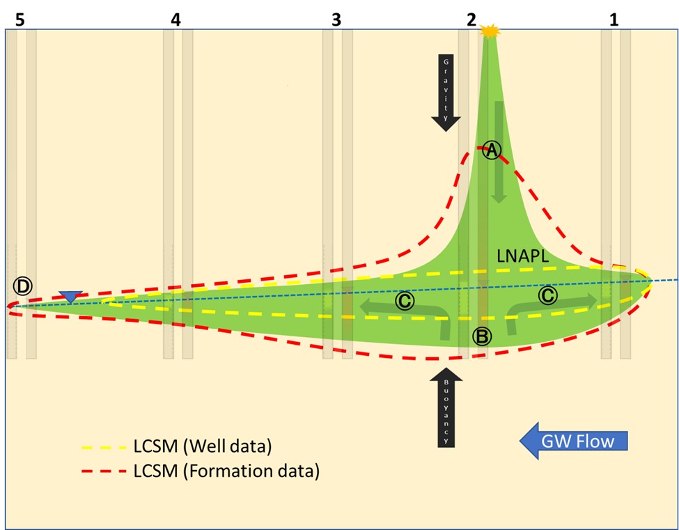
A. Site soil is remarkably homogenous and readily conducts fluids.
B. GW table surface is sloped down toward the left.
C. LNAPL just below the release point is present in the formation, above the GW surface.
D. LNAPL is present in the formation below the GW surface – deepest observations are directly below the release and the penetration tapers with lateral distance from the release point.
The only mismatch between our LCSMs and reality is the relative size difference, which isn’t enough to significantly affect the risk analysis and subsequent remediation design should one be required. This exercise demonstrates that in the absence of heterogeneity, LNAPL characterization is relatively straightforward, perhaps even boring.
Large Scale – Heterogeneous Soil Example
Let’s now examine Figure 3, which consists of the same scenario with the lone exception of swapping over to a more complicated geology.
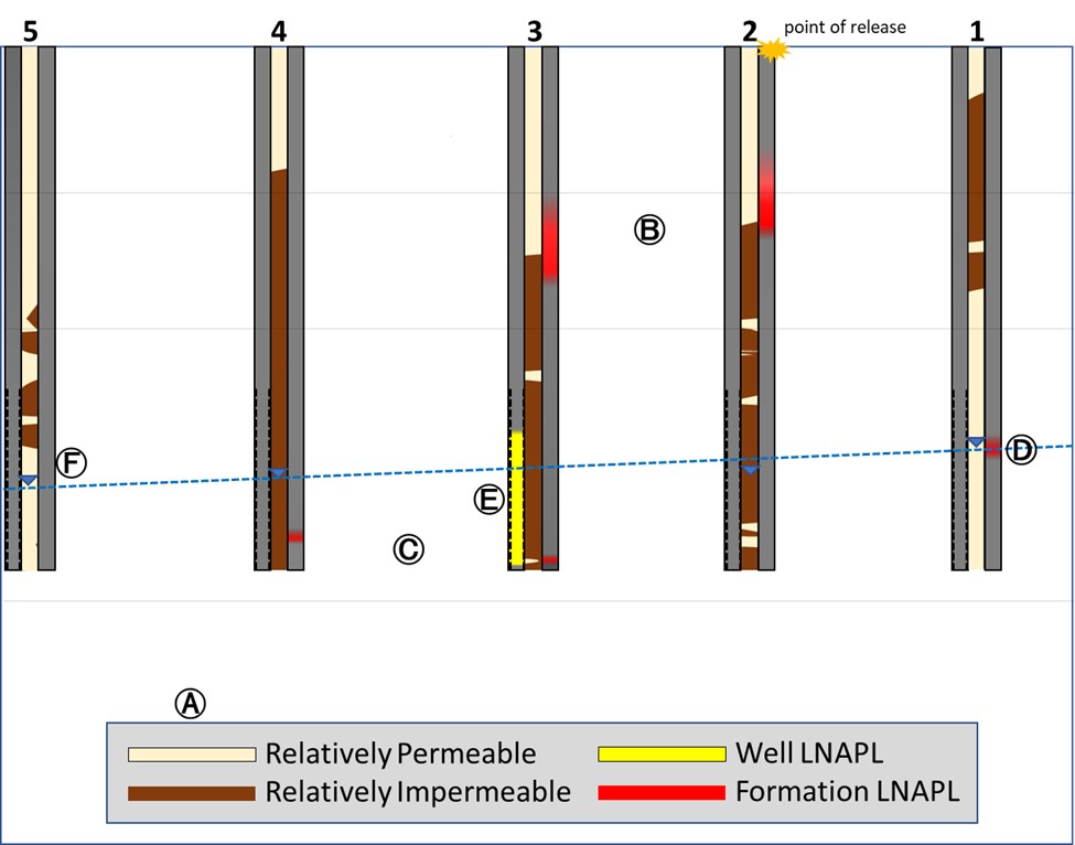
A. Site soils are heterogeneous, differing randomly in their fluid permeability.
B. Formation LNAPL is perched in the vadose zone at some locations, nest #3 perched lower than nest #2.
C. Formation LNAPL is below GW at some locations(nest #3 and nest #4).
D. Formation LNAPL at the GW surface at nest #1.
E. In-well LNAPL is limited to nest #3 and greatly exaggerated in comparison to the formation.
OK, now draw the “LNAPL extent” lines and then let’s look at the reveal in Figure 4 below.
Did I mention I do not like this game anymore?
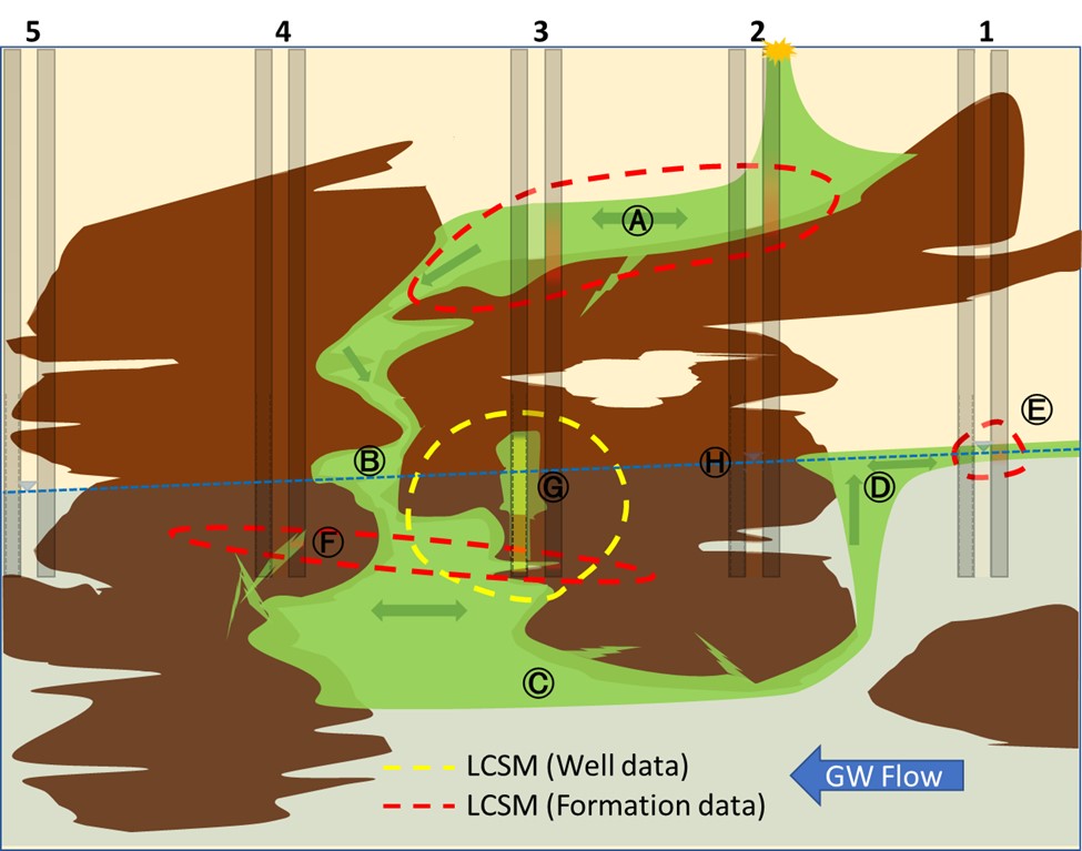
Oh well… let’s autopsy this:
A. We correctly identified the perched LNAPL extent right that was gravity driven to the left – well before it reached GW.
B. An important release chimney (i.e., confined NAPL), straddled by nest #3 and nest #4, was missed. LNAPL pooled and eventually migrated downward, falling into the cavern (area of greater permeability) and pushing far below the GW’s surface.
C. LNAPL eventually filled the impermeable cavern’s ceiling, its buoyancy easily driving it upgradient against the relatively weak forces of GW flow.
D. As a result, LNAPL is now upgradient of the release point at GW surface but at such a low saturation it doesn’t get forced into Well #1.
E. Lone encounter of classic unconfined LNAPL at the water table.
F. LNAPL penetrated low permeability soils, going against intuition (Adamski 2004).
G. Well #3 punctured the cavern ceiling and confined LNAPL flowed into the well, exaggerating its presence.
H. Well #2 doesn’t contain LNAPL because the well screen didn’t span the LNAPL in the formation.
- The formation adjacent to nest #3 contains LNAPL because the well provided a preferential pathway – the investigation itself allowed NAPL to travel where it wouldn’t have if left alone.
- The LNAPL body is continuously connected but our LCSM shows it’s considerably separated.
- The vast majority of the LNAPL body remains hidden to investigators – there doesn’t appear to be troubling levels of LNAPL outside that revealed in Well #3.
- Straddling the GW surface with well screens is a common practice, but this carries the risk of missing significant trapped and perched LNAPL.

Our LCSM doesn’t represent reality very well, but not due to interpretation errors on our part. We were dealt only five narrow strips of information – simply not enough for us to overcome heterogeneity’s countless cloaks and mirages. (Stock 2011)
Small Scale – Heterogeneity Example
Consultants and regulators delineating NAPLs often sample the same location twice. Reasons include:
- Wanting to validate an unproven logging tool’s response by obtaining co-located physical samples during a demonstration/validation project (Einarson 2016).
- Sampling adjacent to a laser-induced fluorescence (LIF) response to determine if a response is truly representative of NAPL versus false positive fluorescence such as wood, calcite, or peat.
- Sampling adjacent to a laser-induced fluorescence (LIF) response in order to relate the LIF response to NAPL saturation (via lab testing of co-located soil/NAPL samples).
- Logging NAPL at the same location twice over a period of time in order to assess changes in NAPL that resulted due to applying a remedy (e.g., dual phase extraction or surfactant enhanced recovery).
- Sampling adjacent to a LIF log that contained an unexpected response that indicated NAPL of a different type than the investigation’s target NAPL. For example, confirming that a diesel signature observed while logging coal tar at a former manufactured gas plant was in fact not coal tar but rather diesel from a previously undocumented diesel release.
To illustrate how heterogeneity introduces uncertainty into repeat sampling at fixed locations, let us conduct an exercise where we’ll repeat NAPL assessments at nest #4, just a foot or two away from the original boring log. Figure 5 contains a few of the many possible outcomes. The original boring log is shown in each panel, while the co-located log(s) are shown alongside in slate blue.
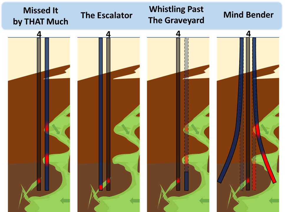
Missed It by THAT Much
The repeat log traveled through different geologic features than the original. If significant time had passed between the logging events, many investigators will naively assume that the differences are due to LNAPL movement. Had the initial log been produced by an unfamiliar (untrusted) tool, investigators will often consider the initial log to be “faulty” because a physical core is inherently more trustworthy. Falsely assuming that the two repeat methods sampled the same soil horizons is frustratingly common and perhaps even the norm.
The Escalator
Preconceptions trick us into thinking every LNAPL encounter was an encounter with a horizontal “layer” of LNAPL even though borings routinely pass through LNAPL features that are wildly tilted, even vertical. In this panel the repeated boring was to the left, not right, of the initial log. Investigators might falsely attribute this to LNAPL migration, the LNAPL has “moved down” – possibly due to GW fluctuation. The LNAPL hasn’t moved down, it’s simply contained within a severely tilted seam of permeable soil.
Whistling Past the Graveyard
Same location as Missed It by THAT Much, but this time targeted sampling (not continuous) was used. The repeat event not only disputes nest #4 (the lower LNAPL is mysteriously gone) but the repeat sampling event also failed to report the two upper LNAPL encounters that would have helped identify the important nearby “chimney” – in other words the repeat generated a false negative of sorts.
Mind Bender
Illusions can also be produced when rod flex occurs. Prior to incorporation of real time inclinometers into their cone penetration test (CPT) probes, CPT operators would suffer from a loss of verticalness (ISO 2022) and their cones would occasionally emerge from nearby ground, during the penetration test!
In-situ logging tools such as LIF or membrane interface probes also employ flexible rods but they are operated without the aid of real time inclinometers. As a result, their data is generally biased “deeper” than the contaminants really are, because the length of rod in the ground often exceeds the probe’s true depth. Combine this depth mirage with the probe travelling laterally and you have the recipe for major hijinks. Only the original log in nest #4 (conducted vertically and straight) represents the LNAPL’s true depth, while the two “benders” resulted in illusions (shown dashed and faded) that would mislead investigators.
A Word of Caution
References
Paul Stock, “Where’s the LNAPL? How about Using LIF to Find It?”, L.U.S.T.Line, pp.13-18
https://neiwpcc.org/wp-content/uploads/2020/07/lustline_68.pdf
Adamski 2004
Adamski, Mark & Kremesec, Victor & Kolhatkar, Ravi & Pearson, Chris & Rowan, Beth. (2005). LNAPL in fine‐grained soils: Conceptualization of saturation, distribution, recovery, and their modeling. Ground Water Monitoring & Remediation. 25. 100 – 112.
https://ngwa.onlinelibrary.wiley.com/doi/abs/10.1111/j.1745-6592.2005.0005.x
Einarson 2016
Einarson, M., Fure, A., St. Germain, R., Chapman, S., and Parker, B., DyeLIF™: A New Direct‐Push Laser‐Induced Fluorescence Sensor System for Chlorinated Solvent DNAPL and Other Non‐Naturally Fluorescing NAPLs. Groundwater Monitoring & Remediation, 38, 3, (28-42), (2018).
https://ngwa.onlinelibrary.wiley.com/doi/abs/10.1111/gwmr.12296
ISO 2022
ISO 22476-1:2022 (Figure 3)
Geotechnical investigation and testing — Field testing — Part 1: Electrical cone and piezocone penetration test
https://www.iso.org/obp/ui/#iso:std:iso:22476:-1:ed-2:v1:en
Research Corner

Postdoctoral Research Associate
Colorado School of Mines
Abstract
Related Links
ANSR Archives
Coming Up
Announcements
Upcoming ITRC Training
- April 13: TRC PFAS Introductory Training
- May 11: Sustainable Resilient Remediation (SRR)
Upcoming IPEC Training
- March 23: Mechanisms for Success in In-Situ Bioremediation Programs and Hydrocarbon Destruction via Biostimulation Alone under Baseline Conditions…
- April 13: Organo-Halide Destruction via Biostimulation Without Augmentation… and Another WOTUS Rule Change?
- April 20: Molecular Biological Tools to Optimize Hydrocarbon Biodegradation and Corrosion Inhibiting Method for Remediating Hydrocarbon Releases at Pipeline, Tank Batteries & AST Sites
- May 4: Hydrocarbon Pipeline Integrity and Changes to Hydrocarbon Components During Composting Study
- May 18: Enhance VOC, Sorbed, Globule, NAPL Remediation Exposing Limiting Factors